19  Working with data at scale

19.1 The awkward middle

You know how to scale web services. You’ve added caches, sharded databases, put queues between components, and split monoliths into microservices. So when someone says “this dataset is too big”, your instinct is to reach for distributed systems — Spark clusters, cloud data warehouses, parallel processing frameworks.

That instinct is often wrong.

Most data science work lives in an awkward middle ground: datasets too large for naive code but far too small to justify a distributed system. A 5 GB CSV that crashes your pandas script doesn’t need Spark — it needs you to understand why pandas is using 40 GB of RAM for 5 GB of data, and how to fix that. A feature engineering pipeline that takes three hours doesn’t need a cluster — it needs vectorised operations instead of Python loops.

If Section 17.1 was about making data flow reliably and Section 18.1 was about making models operational, this chapter is about making both of those processes fast enough on a single machine. The techniques here — memory profiling, dtype selection, vectorisation, chunked processing, and statistical sampling — are the data-processing equivalents of query optimisation and connection pooling. They make an enormous practical difference, and you already understand the principles behind most of them.

19.2 Profiling memory: know before you optimise

The first rule of performance work in any domain is: measure before you change anything. In web services, you’d never optimise a function without profiling it first. The same discipline applies to data processing.

pandas provides a built-in memory profiler. The memory_usage(deep=True) method reports actual memory consumption, including the contents of Python objects — without deep=True, pandas reports only the memory for the pointers, not the strings they point to:

import numpy as np
import pandas as pd

rng = np.random.default_rng(42)
n = 200_000

df = pd.DataFrame({
    "user_id": np.arange(n),
    "event_type": rng.choice(
        ["page_view", "click", "purchase", "scroll", "logout"], n
    ),
    "country": rng.choice(["GB", "US", "DE", "FR", "JP", "AU"], n),
    "response_ms": rng.exponential(120, n),
    "session_id": [f"sess-{i:08d}" for i in rng.integers(0, 50_000, n)],
    "revenue": rng.exponential(25, n).round(2),
    "is_mobile": rng.choice([True, False], n),
})

# Force Python-object string storage to demonstrate the overhead you'll
# encounter with older pandas versions, CSV imports with dtype="object",
# and many third-party libraries that return Python strings.
# pandas 3.0+ defaults to Arrow strings for new DataFrames — see note below.
for col in ["event_type", "country", "session_id"]:
    df[col] = df[col].astype(object)

# Shallow vs deep memory usage
shallow = df.memory_usage(deep=False).sum() / 1024**2
deep = df.memory_usage(deep=True).sum() / 1024**2
print(f"Shallow (pointer-only): {shallow:.1f} MB")
print(f"Deep (actual):          {deep:.1f} MB")
print(f"Ratio:                  {deep / shallow:.1f}×")
print()
print(df.dtypes)

Shallow (pointer-only): 9.3 MB
Deep (actual):          37.0 MB
Ratio:                  4.0×

user_id          int64
event_type      object
country         object
response_ms    float64
session_id      object
revenue        float64
is_mobile         bool
dtype: object

The gap between shallow and deep usage reveals the core problem with Python-object string storage. Each Python string carries a base overhead of roughly 41 bytes (type pointer, reference count, hash, length) plus 1 byte per ASCII character. For a 2-character country code like "GB", the total memory is 43 bytes — over 20× the actual data. For short, repetitive strings like country codes and event types, this overhead dwarfs the data itself.

Numeric columns are efficient — they’re stored as contiguous NumPy arrays of fixed-width values. A column of float64 uses exactly 8 bytes per value, no overhead. The problem is almost always the object-dtype columns.

A note on pandas versions: pandas 3.0 and later defaults to Arrow-backed string storage, which eliminates the Python-object overhead described above. If you’re running pandas 3.0+, string columns in new DataFrames will already be stored efficiently. We force object dtype here to demonstrate the pattern you’ll encounter in existing codebases, when loading CSVs with explicit dtype='object', and when working with libraries that return Python strings. The optimisation techniques in the next section remain valuable regardless — categoricals still provide a 90%+ reduction over Arrow strings for low-cardinality columns, and numeric downcasting helps across all versions.

19.3 Dtype optimisation

Understanding memory layout points directly to the fix: use narrower types. This is the same principle as choosing INT vs BIGINT in a database schema, but with more dramatic effects because pandas defaults to the widest types.

Three techniques cover most cases: numeric downcasting, categorical encoding, and Arrow-backed strings.

Numeric downcasting replaces wide types with narrower ones that still fit the data. A column of non-negative integers between 0 and 255 doesn’t need 8 bytes per value (int64); a single byte (uint8) will do. For signed values in the range –128 to 127, int8 is the corresponding choice:

df_opt = df.copy()

# Downcast numerics where safe
df_opt["user_id"] = pd.to_numeric(df_opt["user_id"], downcast="unsigned")
df_opt["response_ms"] = pd.to_numeric(df_opt["response_ms"], downcast="float")
df_opt["revenue"] = pd.to_numeric(df_opt["revenue"], downcast="float")
df_opt["is_mobile"] = df_opt["is_mobile"].astype("bool")

# Low-cardinality strings → Categorical
df_opt["event_type"] = df_opt["event_type"].astype("category")
df_opt["country"] = df_opt["country"].astype("category")

# High-cardinality strings → PyArrow strings (requires the pyarrow package,
# already in our dependencies for Parquet support)
df_opt["session_id"] = df_opt["session_id"].astype("string[pyarrow]")

deep_before = df.memory_usage(deep=True).sum() / 1024**2
deep_after = df_opt.memory_usage(deep=True).sum() / 1024**2

print(f"Before: {deep_before:.1f} MB")
print(f"After:  {deep_after:.1f} MB")
print(f"Saved:  {(1 - deep_after / deep_before) * 100:.0f}%")
print()
print(df_opt.dtypes)

Before: 37.0 MB
After:  6.9 MB
Saved:  81%

user_id          uint32
event_type     category
country        category
response_ms     float32
session_id       string
revenue         float32
is_mobile          bool
dtype: object

Categorical columns are the big win for low-cardinality strings. Instead of storing the string "page_view" 40,000 times, pandas stores it once in a lookup table and uses integer codes for each row. For a column with 5 unique values across 200,000 rows, this reduces memory by roughly 90–95%, depending on string length. It’s the same technique as dictionary encoding in columnar databases like Parquet.

Arrow-backed strings (string[pyarrow]) replace Python object storage with Apache Arrow’s native string representation. This eliminates the per-string Python overhead and stores string data in typed buffers rather than as individual Python objects. The pyarrow library makes this available with a single dtype cast.

A word of caution on numeric downcasting: float32 has roughly 7 significant digits of precision. For individual measurements like response times this is more than adequate, but for financial columns where exact totals matter — revenue, transaction amounts, account balances — prefer float64. Rounding errors from float32 accumulate when aggregating millions of values, and a sum that’s off by a few pounds is unacceptable in a finance pipeline.

Engineering Bridge

Choosing dtypes deliberately is the DataFrame equivalent of database schema design. In SQL, you’d never use TEXT for a column that only holds country codes — you’d use CHAR(2) or a foreign key to a lookup table. The same thinking applies here: category is the lookup table, float32 is the narrower numeric type, and Arrow strings are the native string store.

The difference is that databases force you to specify types upfront, while pandas infers them lazily (and usually infers the most expensive option). Treating dtype selection as a conscious design decision — the same way you’d design a table schema — prevents most memory problems before they start.

19.4 Vectorisation: why loops betray you

If you’ve profiled a slow pandas pipeline, there’s a good chance the bottleneck is a Python loop disguised as a DataFrame operation. The worst offender is df.apply(lambda row: ..., axis=1) — it looks like a pandas operation, but it’s secretly iterating through rows in pure Python.

To understand why this matters, you need to understand how NumPy executes. When you write df["revenue"] * 1.2, NumPy doesn’t loop through each value in Python. It passes a pointer to the underlying C array to a compiled C function that processes the entire column in a single call. The Python interpreter is involved exactly once — to dispatch the operation — and then C takes over. (The term “vectorised” here refers to this dispatch-to-C pattern; NumPy also uses hardware SIMD instructions internally where available, but the main speedup comes from avoiding the Python interpreter loop.)

When you write df.apply(lambda row: row["revenue"] * 1.2, axis=1), Python calls your lambda function 200,000 times, each time extracting a value, performing the multiplication in Python, and storing the result. The C array is never used as an array; it’s unpacked element by element.

The difference is not subtle:

import time

n_rows = 200_000
data = pd.DataFrame({
    "revenue": rng.exponential(25, n_rows),
    "quantity": rng.integers(1, 20, n_rows),
    "tax_rate": rng.choice([0.0, 0.05, 0.10, 0.20], n_rows),
})

# --- Approach 1: Python loop via apply ---
start = time.perf_counter()
result_loop = data.apply(
    lambda row: row["revenue"] * row["quantity"] * (1 + row["tax_rate"]),
    axis=1,
)
time_loop = time.perf_counter() - start

# --- Approach 2: Vectorised ---
start = time.perf_counter()
result_vec = data["revenue"] * data["quantity"] * (1 + data["tax_rate"])
time_vec = time.perf_counter() - start

print(f"apply (row-wise): {time_loop:.3f}s")
print(f"Vectorised:       {time_vec:.4f}s")
print(f"Speedup:          {time_loop / time_vec:.0f}×")

# Verify they produce the same result
assert np.allclose(result_loop.values, result_vec.values)

apply (row-wise): 1.440s
Vectorised:       0.0027s
Speedup:          526×

The vectorised version is typically 50–200× faster (the exact ratio depends on the hardware and Python version running this code), and the gap widens with larger data. This isn’t a micro-optimisation; it’s the difference between a pipeline that takes three hours and one that takes one minute.

The principle extends beyond arithmetic. Boolean indexing (df[df["country"] == "GB"]), string methods (df["name"].str.lower()), and aggregations (df.groupby("country")["revenue"].sum()) are all vectorised. The rule of thumb: if you’re writing a for loop or apply over a DataFrame, there’s almost certainly a vectorised alternative.

When there isn’t — when the logic genuinely requires row-by-row conditionals — NumPy’s np.where and np.select cover most remaining cases:

# Conditional logic without a loop
data["total"] = np.where(
    data["tax_rate"] > 0,
    data["revenue"] * data["quantity"] * (1 + data["tax_rate"]),
    data["revenue"] * data["quantity"],  # tax-exempt
)

# Multiple conditions with np.select
conditions = [
    data["total"] > 500,
    data["total"] > 100,
]
choices = ["high", "medium"]
data["tier"] = np.select(conditions, choices, default="low")

print(data["tier"].value_counts())

tier
medium    87387
low       79331
high      33282
Name: count, dtype: int64

19.5 Chunked processing

Sometimes the data genuinely doesn’t fit in memory, even with optimised dtypes. A 50 GB log file will not load into a 16 GB laptop regardless of how cleverly you cast columns. The solution is chunked processing: read the data in manageable pieces, process each piece, and combine the results.

pandas supports this natively through the chunksize parameter in read_csv:

import tempfile
import os

# Create a CSV file to demonstrate chunked reading
temp_path = os.path.join(tempfile.gettempdir(), "large_events.csv")
big_df = pd.DataFrame({
    "user_id": rng.integers(0, 100_000, 500_000),
    "event_type": rng.choice(["view", "click", "purchase"], 500_000),
    "revenue": rng.exponential(15, 500_000).round(2),
    "country": rng.choice(["GB", "US", "DE", "FR"], 500_000),
})
big_df.to_csv(temp_path, index=False)

# --- Chunked aggregation ---
country_totals = {}
rows_processed = 0

for chunk in pd.read_csv(temp_path, chunksize=100_000):
    # Aggregate purchases only
    purchases = chunk[chunk["event_type"] == "purchase"]
    for country, total in purchases.groupby("country")["revenue"].sum().items():
        country_totals[country] = country_totals.get(country, 0) + total

    rows_processed += len(chunk)

print(f"Processed {rows_processed:,} rows in chunks")
print("\nRevenue by country (purchases only):")
for country, total in sorted(country_totals.items()):
    print(f"  {country}: £{total:,.2f}")

# Clean up
os.remove(temp_path)

Processed 500,000 rows in chunks

Revenue by country (purchases only):
  DE: £625,738.80
  FR: £627,749.94
  GB: £621,811.93
  US: £623,894.66

The pattern is straightforward: the for chunk in pd.read_csv(...) iterator yields DataFrames of chunksize rows each, and you accumulate results across chunks. The key constraint is that your aggregation must be decomposable — you need to be able to combine partial results. Sums, counts, and means (via sum and count) decompose naturally. Medians and quantiles do not — you’d need to collect all values first, which defeats the purpose. Approximate methods such as t-digest exist for streaming quantile estimation, which Exercise 4 explores.

This is the same pattern as a stateful stream processor: consume records in bounded batches, update running aggregates, discard the batch. The chunksize parameter controls the memory/speed trade-off: smaller chunks use less memory but incur more I/O overhead.

Author’s Note

When I first hit memory limits with pandas, my instinct was to spin up a Spark cluster. It took me an embarrassingly long time to discover that dtype optimisation and chunked processing would have solved 90% of my problems on my laptop. The tooling ecosystem pushes you towards “big data” solutions before you’ve exhausted “medium data” techniques — partly because vendors have an incentive to sell clusters, and partly because blog posts about Spark are more impressive than blog posts about pd.to_numeric(downcast="float").

The lesson: always profile first, optimise dtypes second, try chunked processing third, and reach for distributed tools only after all three have failed. Most data science datasets are not “big data”. They’re medium data with big overhead.

19.6 When less data is the right answer

So far we’ve been asking how to process all the data efficiently. But sometimes the better question is whether you need all of it at all.

Engineers tend to assume that more data is always better. In software, that’s often true — you want complete logs, full test coverage, every transaction recorded. But in data science, the relationship between dataset size and analytical value has sharply diminishing returns, and understanding when you can use a sample saves enormous time and money.

The statistical foundation comes from the margin of error for an estimated proportion, which we explored in Section 6.4:

\[ \text{Margin of error} \approx z \sqrt{\frac{\hat{p}(1 - \hat{p})}{n}} \]

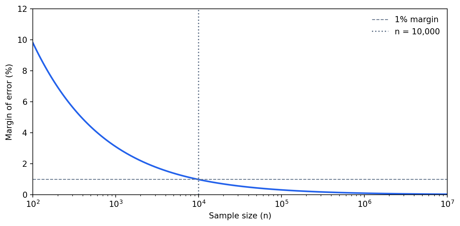
Here \(z\) is the critical value from the standard normal distribution (1.96 for 95% confidence), \(\hat{p}\) is the estimated proportion, and \(n\) is the sample size. The worst case (\(\hat{p} = 0.5\)) at 95% confidence gives roughly \(0.98 / \sqrt{n}\). For a sample of 10,000 rows, that’s about 1 percentage point. For 100,000 rows, it’s about 0.3 percentage points. Going from 100,000 to 10,000,000 rows improves precision from 0.3% to 0.03% — almost never meaningful for business decisions.

import matplotlib.pyplot as plt

sample_sizes = np.logspace(2, 7, 200)  # 100 to 10 million
margin_of_error = 1.96 * np.sqrt(0.25 / sample_sizes)  # worst-case p=0.5

fig, ax = plt.subplots(figsize=(8, 4))
ax.plot(sample_sizes, margin_of_error * 100, color="#2563eb", linewidth=2)
ax.set_xscale("log")
ax.set_xlabel("Sample size (n)")
ax.set_ylabel("Margin of error (%)")
ax.axhline(y=1, color="#64748b", linestyle="--", linewidth=1, label="1% margin")
ax.axvline(x=10_000, color="#64748b", linestyle=":", linewidth=1.5, label="n = 10,000")
ax.legend(frameon=False)
ax.set_xlim(100, 1e7)
ax.set_ylim(0, 12)
plt.tight_layout()
plt.show()

Figure 19.1: At n = 10,000 the margin of error is already below 1%. Scaling to 10 million rows improves precision by less than 0.3 percentage points — rarely worth the cost.

This means that for aggregate statistics — means, proportions, correlations — a random sample of 10,000–50,000 rows gives you nearly all the precision you’ll ever need. Processing 10 million rows to compute a mean is not 1,000× more informative; it’s barely more informative at all.

# Generate a large dataset
full_data = pd.DataFrame({
    "revenue": rng.exponential(50, 1_000_000),
    "is_mobile": rng.choice([True, False], 1_000_000, p=[0.6, 0.4]),
    "country": rng.choice(["GB", "US", "DE", "FR"], 1_000_000),
})

# Compare full computation vs sample
full_mean = full_data["revenue"].mean()
full_mobile_pct = full_data["is_mobile"].mean()
full_country = full_data.groupby("country")["revenue"].mean()

sample = full_data.sample(10_000, random_state=42)
sample_mean = sample["revenue"].mean()
sample_mobile_pct = sample["is_mobile"].mean()
sample_country = sample.groupby("country")["revenue"].mean()

# Build a comparison table
country_comp = pd.DataFrame({
    "Full (1M rows)": full_country,
    "Sample (10K rows)": sample_country,
})
country_comp["Relative error (%)"] = (
    (country_comp["Full (1M rows)"] - country_comp["Sample (10K rows)"]).abs()
    / country_comp["Full (1M rows)"] * 100
)

print(f"Mean revenue — full: {full_mean:.2f}, sample: {sample_mean:.2f}, "
      f"error: {abs(full_mean - sample_mean) / full_mean * 100:.2f}%")
print(f"Mobile %     — full: {full_mobile_pct:.4f}, sample: {sample_mobile_pct:.4f}, "
      f"error: {abs(full_mobile_pct - sample_mobile_pct) / full_mobile_pct * 100:.2f}%")
print("\nRevenue by country:")
country_comp.round(2)

Mean revenue — full: 49.96, sample: 50.14, error: 0.36%
Mobile %     — full: 0.5998, sample: 0.5960, error: 0.64%

Revenue by country:

	Full (1M rows)	Sample (10K rows)	Relative error (%)
country
DE	49.91	49.67	0.49
FR	50.21	50.15	0.13
GB	49.96	51.37	2.82
US	49.77	49.41	0.73

The errors are typically well under 2%, and the sample was computed on 1% of the data.

However, sampling is dangerous when you care about rare events or tail behaviour. If only 0.1% of transactions are fraudulent, a random sample of 10,000 rows contains roughly 10 fraud cases — too few to train a model or compute stable statistics. Similarly, if you need the 99th percentile of response times, you need enough data in the tail to estimate it precisely. For these cases, stratified sampling (oversampling the rare class) or working with the full dataset is necessary.

One further caveat: the margins above assume a simple random sample from an exchangeable population. If rows are clustered — for example, multiple events per user where individual users behave very differently — a simple random sample of 10,000 rows may be less informative than it appears. The effective sample size depends on within-cluster correlation, and stratified or cluster-aware sampling may be needed.

19.7 Lazy evaluation and modern alternatives

pandas is an eager execution engine: every operation runs immediately and returns a result. When you write df[df["country"] == "GB"].groupby("event_type")["revenue"].mean(), pandas creates an intermediate DataFrame for the filter, then another for the groupby, then another for the mean. Each intermediate result occupies memory and takes time to compute.

If you’ve used lazy evaluation in functional programming — Haskell’s thunks, Java’s streams, Kotlin’s sequences — you’ll recognise the alternative. Build a description of the computation first, then execute it all at once. This allows the engine to optimise the execution plan before running anything, the same way a SQL database optimises a query before executing it.

Polars is a DataFrame library built on this principle. Instead of executing operations eagerly, a Polars lazy frame records the sequence of operations and optimises them when you call .collect(). The optimiser can push filters before joins (so you process fewer rows), project only the columns you need (so you read less data), and parallelise independent operations across CPU cores.

The syntax is similar enough to pandas that the transition is straightforward, though the API names differ in places (notably .group_by() instead of pandas’s .groupby()):

# Polars (not executed — illustrative only)
import polars as pl

result = (
    pl.scan_csv("events.csv")          # lazy: no data read yet
    .filter(pl.col("country") == "GB")  # recorded, not executed
    .group_by("event_type")             # recorded, not executed
    .agg(pl.col("revenue").mean())      # recorded, not executed
    .collect()                          # NOW: optimise and execute
)

Polars offers several concrete advantages over pandas. Query optimisation pushes filters before joins, so unnecessary rows are never loaded from disk, and column projection means only required columns are read. Execution is parallel by default — Polars uses all CPU cores where pandas is single-threaded for most operations. Strings are Arrow-backed natively, eliminating the Python object overhead without any manual dtype conversion. And Polars copies data less aggressively than pandas, reducing peak memory usage for complex pipelines.

You don’t need Polars to be productive at scale — everything earlier in this chapter works with pandas alone. But as datasets grow beyond a few gigabytes, or as pipelines become complex enough that query optimisation matters, Polars offers genuine engineering advantages.

Engineering Bridge

The eager-vs-lazy distinction in DataFrame libraries maps directly to a pattern every backend engineer knows: the difference between executing SQL statements one at a time and composing a query that the database optimiser can plan holistically. An eager DataFrame is like issuing SELECT * FROM events, filtering the result in application code, then joining with another table in application code. A lazy DataFrame is like writing a single query with WHERE, JOIN, and GROUP BY and letting the query planner choose the execution order. The same data, the same result — but the lazy version can be orders of magnitude faster because the optimiser sees the full picture.

19.8 Worked example: optimising a pipeline

Let’s put these techniques together. We’ll simulate a typical data science task — computing feature statistics from a web analytics dataset — and optimise it step by step.

import time

# Generate a realistic web analytics dataset
n = 500_000
analytics = pd.DataFrame({
    "user_id": [f"user-{i:06d}" for i in rng.integers(0, 50_000, n)],
    "page": rng.choice(
        ["/home", "/products", "/cart", "/checkout", "/account",
         "/search", "/help", "/about"],
        n,
    ),
    "device": rng.choice(["desktop", "mobile", "tablet"], n, p=[0.4, 0.5, 0.1]),
    "timestamp": (
        pd.Timestamp("2024-01-01")
        + pd.to_timedelta(rng.uniform(0, 30 * 24 * 3600, n), unit="s")
    ),
    "response_ms": rng.exponential(150, n),
    "bytes_sent": rng.lognormal(10, 1.2, n).astype(int),
    "is_error": rng.choice([0, 1], n, p=[0.97, 0.03]),
})

# Force object dtype on strings for a clear baseline
for col in ["user_id", "page", "device"]:
    analytics[col] = analytics[col].astype(object)

baseline_mb = analytics.memory_usage(deep=True).sum() / 1024**2
print(f"Baseline memory: {baseline_mb:.1f} MB")
print(f"Dtypes:\n{analytics.dtypes}")

Baseline memory: 96.9 MB
Dtypes:
user_id                object
page                   object
device                 object
timestamp      datetime64[ns]
response_ms           float64
bytes_sent              int64
is_error                int64
dtype: object

That’s the starting point — all string columns stored as Python objects, all numerics at their widest types. Now let’s optimise the dtypes:

opt = analytics.copy()

# Strings → appropriate types
opt["user_id"] = opt["user_id"].astype("string[pyarrow]")
opt["page"] = opt["page"].astype("category")
opt["device"] = opt["device"].astype("category")

# Numerics → narrower types
opt["response_ms"] = pd.to_numeric(opt["response_ms"], downcast="float")
opt["bytes_sent"] = pd.to_numeric(opt["bytes_sent"], downcast="unsigned")
opt["is_error"] = opt["is_error"].astype("bool")

optimised_mb = opt.memory_usage(deep=True).sum() / 1024**2
print(f"Optimised memory: {optimised_mb:.1f} MB")
print(f"Reduction:        {(1 - optimised_mb / baseline_mb) * 100:.0f}%")
print(f"\nDtypes:\n{opt.dtypes}")

Optimised memory: 18.1 MB
Reduction:        81%

Dtypes:
user_id                string
page                 category
device               category
timestamp      datetime64[ns]
response_ms           float32
bytes_sent             uint32
is_error                 bool
dtype: object

The timestamp column (datetime64[ns]) is already at its narrowest practical representation — 8 bytes per value with nanosecond precision. No further optimisation needed there.

Now let’s compute error rates by page and device using the optimised DataFrame:

# groupby aggregation on the optimised DataFrame
start = time.perf_counter()
summary = (
    opt.groupby(["page", "device"])
    .agg(
        total_requests=("is_error", "count"),
        error_count=("is_error", "sum"),
        mean_response=("response_ms", "mean"),
        p95_response=("response_ms", lambda x: x.quantile(0.95)),
    )
)
summary["error_rate"] = summary["error_count"] / summary["total_requests"]
time_vectorised = time.perf_counter() - start

print(f"Groupby completed in: {time_vectorised:.3f}s")
print("\nTop 5 page/device combinations by error rate:")
summary.nlargest(5, "error_rate")[["total_requests", "error_rate", "mean_response"]]

Groupby completed in: 0.084s

Top 5 page/device combinations by error rate:

		total_requests	error_rate	mean_response
page	device
/home	tablet	6271	0.033169	154.420349
/search	tablet	6193	0.033102	149.541611
/help	desktop	24909	0.031675	149.223038
/products	mobile	31486	0.031030	151.922241
/home	mobile	31267	0.030863	149.840836

Note that the lambda for the 95th percentile forces pandas to call Python per group, bypassing its internal C-optimised aggregation path. For the built-in aggregations (count, sum, mean), pandas uses fast C code. When every millisecond matters, computing quantiles separately via .groupby(...)[col].quantile(0.95) avoids the per-group Python overhead.

Finally, let’s demonstrate that sampling gives us the same insights at a fraction of the cost:

# Same analysis on a 5% sample
sample_opt = opt.sample(frac=0.05, random_state=42)

start = time.perf_counter()
sample_summary = (
    sample_opt.groupby(["page", "device"])
    .agg(
        total_requests=("is_error", "count"),
        error_count=("is_error", "sum"),
        mean_response=("response_ms", "mean"),
    )
)
sample_summary["error_rate"] = (
    sample_summary["error_count"] / sample_summary["total_requests"]
)
time_sampled = time.perf_counter() - start

# Compare error rates between full and sampled
comparison = summary[["error_rate"]].join(
    sample_summary[["error_rate"]], rsuffix="_sample"
)
comparison["abs_diff"] = (
    (comparison["error_rate"] - comparison["error_rate_sample"]).abs()
)

print(f"Sampled groupby:  {time_sampled:.4f}s")
print(f"Mean absolute difference in error rates: "
      f"{comparison['abs_diff'].mean():.4f}")
print(f"Max absolute difference in error rates:  "
      f"{comparison['abs_diff'].max():.4f}")

Sampled groupby:  0.0092s
Mean absolute difference in error rates: 0.0042
Max absolute difference in error rates:  0.0163

The sampled analysis produces nearly identical error rates — the differences are in the noise — while using 5% of the data.

19.9 Summary

Working with data at scale is less about big infrastructure and more about understanding your tools:

1. Profile first. Use memory_usage(deep=True) to understand where memory goes. Object-dtype columns (strings) are almost always the main offender.

2. Choose types deliberately. Categoricals for low-cardinality strings, Arrow strings for high-cardinality, and numeric downcasting for numbers. Memory reductions of 40% or more are typical, with higher gains when columns are predominantly low-cardinality strings.

3. Vectorise everything. A single vectorised operation replaces 200,000 Python function calls. If you’re writing apply with axis=1, you’re almost certainly doing it wrong.

4. Chunk when you must. For data that genuinely exceeds memory, chunked reading with incremental aggregation handles most use cases. Ensure your aggregation is decomposable.

5. Sample when you can. For aggregate statistics, 10,000 rows give you 1% precision. Processing millions of extra rows rarely adds analytical value — though rare events and clustered data require more care.

The techniques here apply regardless of what comes next in your pipeline — whether that’s the model deployment patterns from Section 18.1 or the testing strategies we’ll explore in Testing Data Science Code.

19.10 Exercises

Exercise 1. Write a function optimise_dtypes(df: pd.DataFrame) -> pd.DataFrame that automatically optimises a DataFrame’s memory usage. For each column: downcast numeric types, convert object columns with fewer than 50 unique values to category, and convert remaining object columns to string[pyarrow]. Return the optimised DataFrame and print the before/after memory usage.

Exercise 2. Using the analytics DataFrame from the worked example (which includes a timestamp column), write a groupby aggregation that computes, for each user_id, the number of sessions (defined as sequences of events more than 30 minutes apart), the total pages visited, and the mean response time. Do this without using apply. Hint: think about how to detect session boundaries using vectorised time differences within each user’s sorted events.

Exercise 3. Using the margin of error formula, calculate the minimum sample size needed to estimate a proportion within ±0.5 percentage points at 95% confidence (worst-case \(\hat{p} = 0.5\)). Then verify empirically: generate a population of 10 million Bernoulli trials with \(p = 0.3\), draw 1,000 random samples of that size, and check what fraction of the sample proportions fall within 0.5 percentage points of the true value.

Exercise 4. Adapt the chunked processing pattern to compute the median revenue across a dataset that doesn’t fit in memory. Explain why the naive approach (accumulating all values across chunks) defeats the purpose of chunking, and propose an approximate alternative. Hint: research the t-digest algorithm or consider using a histogram-based approximation. Where does the analogy to decomposable aggregations break down?

Exercise 5. A colleague argues that they should always load complete datasets because “you never know what you’ll need later in the analysis.” Write a brief counter-argument (3–5 sentences), drawing on both the statistical argument about diminishing returns and the engineering argument about resource costs. Under what circumstances is your colleague actually right?