---
# Content: CC BY-NC-SA 4.0 | Code: MIT - see /LICENSE.md
title: "Linear regression: your first model"
---
{{< include /_common-imports.qmd >}}
## From description to prediction {#sec-from-description-to-prediction}
Parts 1 and 2 gave you the tools to describe data and draw inferences from it. You can summarise a distribution, test a hypothesis, and quantify your uncertainty about a parameter. These are powerful capabilities, but they're fundamentally backward-looking. They tell you about data you've already collected.
This chapter marks a turn. In Part 3, we start *building models*: mathematical functions that capture the relationship between inputs and outputs so you can predict outcomes you haven't yet observed. The simplest, most interpretable, and most important of these models is **linear regression**.
If you've ever eyeballed a scatter plot and thought "there's a trend there," you've already done regression informally. If you've estimated how long a deployment will take based on the number of services being updated, you've done it mentally. Linear regression is the formal version: it finds the line (or hyperplane, a flat surface generalised to higher dimensions) that best fits your data, tells you how confident you should be in that fit, and gives you a principled way to make predictions.
It also connects everything from Parts 1 and 2. Remember the data-generating process from @sec-dgp: $y = f(x) + \varepsilon$. Linear regression is the special case where $f(x)$ is a straight line. The $\varepsilon$ term — that irreducible noise we met in @sec-determinism — is what keeps the model honest. The hypothesis testing machinery from @sec-hypothesis-testing tells us whether each predictor matters. Confidence intervals from @sec-confidence-intervals quantify our uncertainty about the coefficients. Everything converges here.
A quick note on terminology. Statistics calls the input variables **predictors** (or, in older texts, *regressors* or *independent variables*); machine learning calls them **features**. They refer to the same thing. This book uses *predictors* through the regression chapters, where the statistical vocabulary reads most naturally, and switches to *features* from Chapter 11 onward when we move to tree-based, regularised, and unsupervised methods where the ML vocabulary dominates. The concept doesn't change when the word does.
## The simplest model: one predictor, one line {#sec-simple-regression}
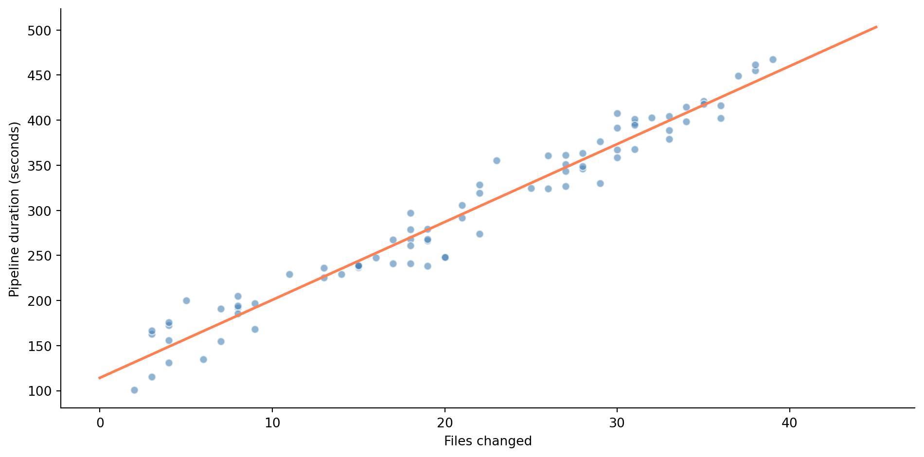
Your CI pipeline runs on every pull request. Some PRs take 2 minutes to build; others take 8. You suspect the duration depends on how many files were changed: more files means more tests to run, more linting to check, more artefacts to build. Let's see if the data supports that intuition.
```{python}
#| label: fig-pipeline-scatter
#| echo: true
#| fig-cap: "CI pipeline duration vs files changed in a pull request. Each point is one build. The orange line is the best-fit line found by ordinary least squares."
#| fig-alt: "Scatter plot of 80 data points showing CI pipeline duration in seconds on the vertical axis and number of files changed on the horizontal axis. Points trend upward from about 120 seconds at 1 file to about 450 seconds at 39 files, with an orange best-fit line running through the cloud of points."
rng = np.random.default_rng(42)

n = 80
files_changed = rng.integers(1, 40, size=n)
pipeline_duration = 120 + 8.5 * files_changed + rng.normal(0, 25, size=n)

fig, ax = plt.subplots(figsize=(10, 5))
fig.patch.set_alpha(0)
ax.patch.set_alpha(0)
ax.scatter(files_changed, pipeline_duration, alpha=0.6, color='#0072B2',
           edgecolor='white')

# Best-fit line (we'll explain how this is computed shortly)
slope, intercept = np.polyfit(files_changed, pipeline_duration, 1)
x_line = np.array([files_changed.min(), files_changed.max()])
ax.plot(x_line, intercept + slope * x_line, '#E69F00', linewidth=2)

ax.set_xlabel('Files changed')
ax.set_ylabel('Pipeline duration (seconds)')
ax.spines[['top', 'right']].set_visible(False)
plt.tight_layout()
plt.show()
```
@fig-pipeline-scatter shows the relationship: noisy, but with a clear upward trend captured by the fitted line. A 10-file PR might take anywhere from 150 to 250 seconds, but on average, more files means longer builds. The line gives us a concrete prediction for any PR size. But how did we find this particular line? What makes it the "best" one?
"Best" needs a definition. Linear regression defines it as the line that minimises the **residual sum of squares** (RSS), the total squared vertical distance between each observed point and the line's prediction. If our line predicts $\hat{y}_i$ (read "y-hat"; the hat marks it as an estimated value) for observation $i$ but we actually observed $y_i$, the residual is $e_i = y_i - \hat{y}_i$, and we minimise:
$$
\text{RSS} = \sum_{i=1}^{n} (y_i - \hat{y}_i)^2 = \sum_{i=1}^{n} e_i^2
$$
This method, **ordinary least squares** (OLS), has a closed-form solution. For a model with one predictor, $\hat{y} = \beta_0 + \beta_1 x$ (where $\beta_0$ is the intercept and $\beta_1$ the slope), the optimal coefficients are:
$$
\hat{\beta}_1 = \frac{\sum_{i=1}^{n}(x_i - \bar{x})(y_i - \bar{y})}{\sum_{i=1}^{n}(x_i - \bar{x})^2} = \frac{\text{Cov}(x, y)}{\text{Var}(x)}
$$
$$
\hat{\beta}_0 = \bar{y} - \hat{\beta}_1 \bar{x}
$$
As with $\hat{y}$, the hats on $\hat{\beta}_0$ and $\hat{\beta}_1$ mark them as estimates computed from data; the true coefficients $\beta_0$ and $\beta_1$ remain unknown.
The slope $\hat{\beta}_1$ is the covariance divided by the variance. If you recall from @sec-relationships, the Pearson correlation $r$ is the covariance divided by the product of standard deviations. So $\hat{\beta}_1 = r \cdot (s_y / s_x)$, where $s_x$ and $s_y$ are the standard deviations of $x$ and $y$: the correlation rescaled from standardised units (mean 0, standard deviation 1) to the natural units of the data. The intercept $\hat{\beta}_0$ ensures the line passes through the point $(\bar{x}, \bar{y})$, the sample means of $x$ and $y$ (the bar notation always denotes a mean).
```{python}
#| label: manual-ols
#| echo: true
# Manual OLS calculation
x, y = files_changed, pipeline_duration

beta_1 = np.cov(x, y, ddof=1)[0, 1] / np.var(x, ddof=1)
beta_0 = np.mean(y) - beta_1 * np.mean(x)

print(f"Manual OLS:")
print(f"  Intercept (β₀): {beta_0:.2f} seconds")
print(f"  Slope (β₁):     {beta_1:.2f} seconds per file")
print(f"\nInterpretation:")
print(f"  A PR with 0 files changed would take ~{beta_0:.0f}s (pipeline overhead)")
print(f"  Each additional file adds ~{beta_1:.1f}s to the build")
```
The intercept tells you the baseline pipeline duration: the fixed cost of checkout, environment setup, and core tests even for a trivial change. The slope tells you the marginal cost per file. These aren't just abstract numbers; they map directly to operational decisions. If each file adds roughly 8.5 seconds and your target build time is under 5 minutes, you can estimate the maximum PR size that stays within budget.
::: {.callout-note}
## Engineering Bridge
Some equations have closed-form solutions (the quadratic formula) while others require numerical methods (Newton's method for root-finding). OLS is in the first camp: the loss function (the RSS we defined above) on a linear model has exactly one minimum, and you can solve for it directly. Most machine learning models aren't this fortunate; they rely on an iterative algorithm called **gradient descent**, which takes repeated steps toward the optimum without ever computing it in one shot. It's like having an algebraic formula for the optimal thread pool size instead of benchmarking your way there. When we meet logistic regression in *Logistic regression and classification*, we'll lose this luxury and need iterative solvers.
:::
## Fitting with statsmodels: the full picture {#sec-statsmodels-ols}
The manual calculation gives us the coefficients, but there's much more to extract from a regression. The `statsmodels` library provides the complete statistical picture.
```{python}
#| label: statsmodels-fit
#| echo: true
import statsmodels.api as sm

# statsmodels requires us to add a constant column for the intercept explicitly.
# Here we use a DataFrame for readable column names in the output;
# later we'll use sm.add_constant(), which is more concise for many predictors.
X = pd.DataFrame({'const': 1, 'files_changed': files_changed})
model = sm.OLS(pipeline_duration, X).fit()

print(model.summary())
```
That is a lot of output. Let's unpack the parts that matter.
**Coefficients (`coef`).** The `const` row is $\hat{\beta}_0$ (the intercept); the `files_changed` row is $\hat{\beta}_1$ (the slope). These match our manual calculation.
**Standard errors and confidence intervals.** Each coefficient has a standard error, the standard deviation of its sampling distribution, the same concept we met in @sec-standard-error. The 95% confidence interval tells you the range of plausible true values. If the confidence interval for the slope excludes zero, you have evidence that $x$ genuinely predicts $y$.
**t-statistics and p-values.** The $t$-statistic for each coefficient tests $H_0$: $\beta = 0$ (the predictor has no effect). This is the same t-test logic from @sec-testing-framework: the coefficient divided by its standard error, compared to a t-distribution. A small p-value means the predictor is statistically significant.
**R-squared ($R^2$).** The proportion of variance in $y$ explained by the model. It's defined as:
$$
R^2 = 1 - \frac{\text{RSS}}{\text{TSS}} = 1 - \frac{\sum (y_i - \hat{y}_i)^2}{\sum (y_i - \bar{y})^2}
$$
where TSS (total sum of squares) measures the total variability of $y$ around its mean, the baseline against which the model's improvement is measured. An $R^2$ of 0.96 means the model captures 96% of the variability in pipeline duration; the remaining 4% is noise the model can't explain. In simple regression (with an intercept), $R^2 = r^2$, literally the square of the Pearson correlation from @sec-relationships. See @sec-metrics-index for a quick comparison of $R^2$ with the other evaluation metrics used in this book.
**F-statistic.** The F-statistic tests whether the model as a whole explains statistically significant variance: whether at least one predictor has a non-zero coefficient. It works by comparing how much variance the model explains to how much it leaves unexplained: a large ratio means the model is doing real work, not just fitting noise. With one predictor, the F-test and the t-test on that predictor give identical conclusions. It becomes more useful in multiple regression.
```{python}
#| label: fig-regression-line
#| echo: true
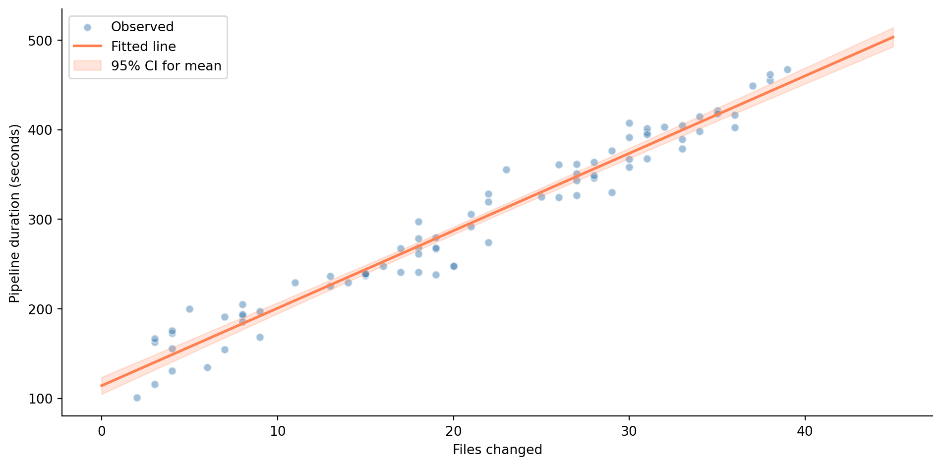
#| fig-cap: "The fitted regression line with a 95% confidence band for the mean prediction (not individual observations). The band is narrowest near the centre of the data and widens towards the extremes."
#| fig-alt: "Scatter plot of CI pipeline duration vs files changed, with an orange regression line running from lower-left to upper-right. A shaded band around the line shows the 95% confidence interval for the mean prediction, narrowest near 20 files and widening towards the edges of the data range."
fig, ax = plt.subplots(figsize=(10, 5))
fig.patch.set_alpha(0)
ax.patch.set_alpha(0)
ax.scatter(files_changed, pipeline_duration, alpha=0.5, color='#0072B2',
           edgecolor='white', label='Observed')

# Prediction with confidence band
x_plot = np.linspace(0, 45, 200)
X_plot = pd.DataFrame({'const': 1, 'files_changed': x_plot})
predictions = model.get_prediction(X_plot)
pred_summary = predictions.summary_frame(alpha=0.05)

ax.plot(x_plot, pred_summary['mean'], '#E69F00', linewidth=2, label='Fitted line')
ax.fill_between(x_plot, pred_summary['mean_ci_lower'], pred_summary['mean_ci_upper'],
                color='#E69F00', alpha=0.2, label='95% CI for mean')

ax.set_xlabel('Files changed')
ax.set_ylabel('Pipeline duration (seconds)')
ax.legend()
ax.spines[['top', 'right']].set_visible(False)
plt.tight_layout()
plt.show()
```
The confidence band in @fig-regression-line shows uncertainty about the *mean response* (the expected value of $y$) at each value of $x$, not where individual observations will fall. It's narrowest near $\bar{x}$ (where we have the most information) and widens as you move towards the edges. This is the regression equivalent of the principle you know from @sec-confidence-intervals: estimates are more precise near the centre of your data.
## Residual analysis: debugging your model {#sec-residual-analysis}
A fitted model is a hypothesis about the data-generating process. Like any hypothesis, it needs testing. In regression, we test it by examining the **residuals**, the differences between what the model predicted and what actually happened. Systematic patterns in the residuals indicate that the model is missing something.
The four key assumptions underlying OLS inference are sometimes remembered by the mnemonic **LINE**. The **L** stands for linearity: the true relationship between $x$ and $y$ is linear. **I** is for independence: the errors (and by extension, the observations) are independent of each other. **N** is for normality: the errors are approximately normally distributed. And **E** is for equal variance, also called homoscedasticity: the errors have constant spread across all values of $x$. When we check these assumptions, we examine the residuals as proxies for the unobservable true errors.
A subtlety worth noting: the coefficient *estimates* are optimal under linearity, exogeneity (the errors have zero mean given the predictor values; the confounding discussion in @sec-regression-pitfalls explains why this matters), equal variance, uncorrelated errors, and no perfect multicollinearity, a result called the **Gauss-Markov theorem**. In plain terms, no other unbiased linear method (one that gets the right answer on average across repeated samples) will produce lower-variance coefficient estimates. Normality is specifically needed for the p-values and confidence intervals to be exact. In practice, all four LINE assumptions are checked together because you usually want both the estimates and the inference.
```{python}
#| label: fig-residual-plots
#| echo: true
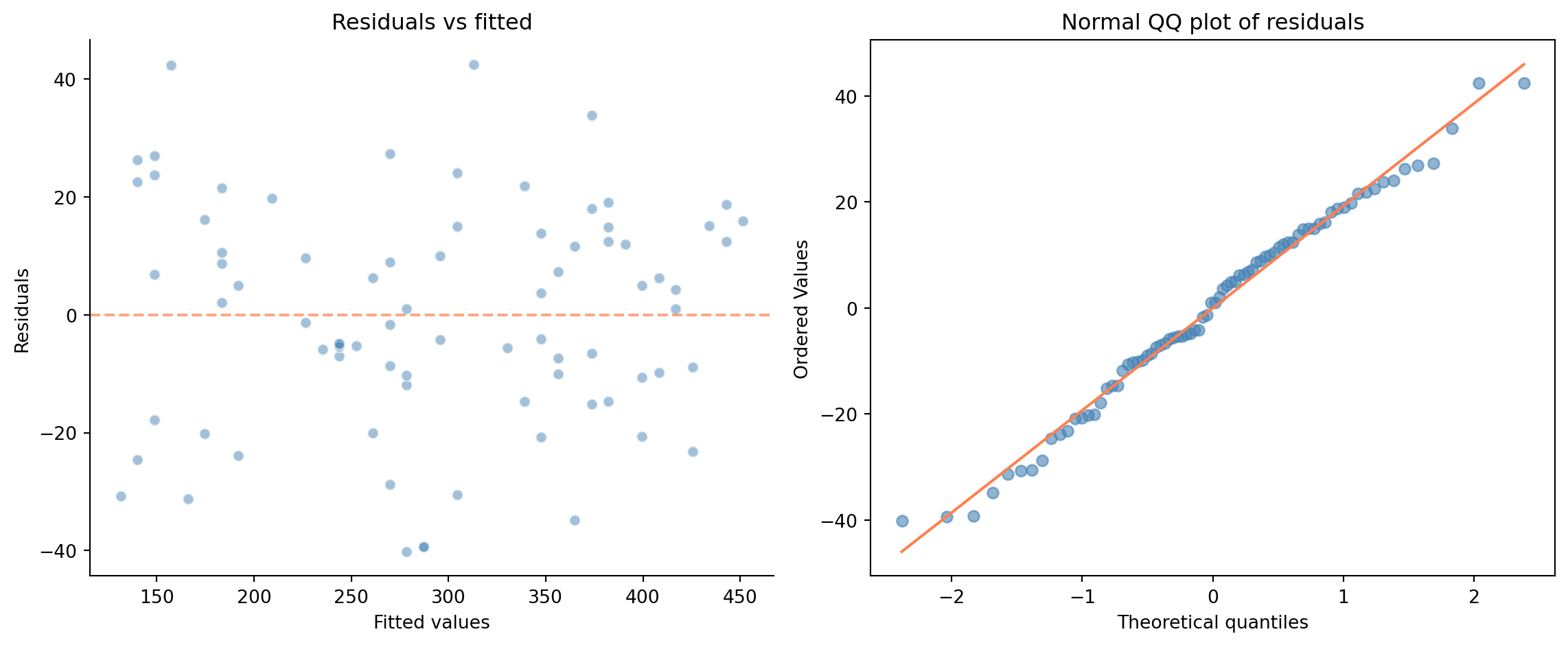
#| fig-cap: "Diagnostic plots for the CI pipeline regression. Left: residuals vs fitted values — no obvious pattern, suggesting linearity and homoscedasticity hold. Right: QQ plot — residuals are approximately normal."
#| fig-alt: "Two-panel diagnostic figure. Left: scatter plot of residuals versus fitted values, showing points randomly scattered around a horizontal line at zero with no discernible pattern or funnel shape. Right: QQ plot of residuals against theoretical normal quantiles, showing points closely following the diagonal reference line."
from scipy import stats

residuals = model.resid
fitted = model.fittedvalues

fig, (ax1, ax2) = plt.subplots(1, 2, figsize=(12, 5))
fig.patch.set_alpha(0)
ax1.patch.set_alpha(0)
ax2.patch.set_alpha(0)

# Residuals vs fitted
ax1.scatter(fitted, residuals, alpha=0.5, color='#0072B2', edgecolor='white')
ax1.axhline(0, color='#E69F00', linestyle='--', alpha=0.7)
ax1.set_xlabel('Fitted values')
ax1.set_ylabel('Residuals')
ax1.set_title('Residuals vs fitted')
ax1.spines[['top', 'right']].set_visible(False)

# QQ plot
stats.probplot(residuals, plot=ax2)
ax2.set_title('Normal QQ plot of residuals')
ax2.get_lines()[0].set_color('#0072B2')
ax2.get_lines()[0].set_alpha(0.6)
ax2.get_lines()[1].set_color('#E69F00')

plt.tight_layout()
plt.show()
```
In @fig-residual-plots, the residuals look well-behaved: no curves, no fan shapes, no outlier clusters. The **QQ plot** (quantile-quantile) on the right compares the distribution of residuals to a theoretical normal distribution: each point plots one residual's observed value against where it would fall if the residuals were perfectly normal. If the points follow the diagonal, normality holds. Here they do, so this model's assumptions appear reasonable, which shouldn't surprise us, since we generated the data to satisfy them. Real data is rarely this clean, and that's precisely when these plots earn their keep.
What would bad residual plots look like? A U-shaped pattern in residuals vs fitted values signals a non-linear relationship: the model is missing a curve. A funnel shape (residuals spreading out as fitted values increase) indicates heteroscedasticity, unequal variance, the violation of the "E" in LINE. Heavy tails in the QQ plot (points curving away from the diagonal at both ends, indicating more extreme values than a normal distribution predicts) suggest the residuals aren't normal, which affects the reliability of p-values and confidence intervals.
::: {.callout-note}
## Engineering Bridge
Residual analysis is debugging for statistical models. Just as you'd examine error logs for patterns — do failures cluster at certain times? Do they correlate with specific inputs? Do they affect certain users disproportionately? — residual plots reveal systematic shortcomings in your model. A random scatter of residuals is the statistical equivalent of "no concerning patterns in the logs." A structured pattern means your model is missing something, and the shape of the pattern often tells you *what*.
:::
## Multiple regression: more predictors, same framework {#sec-multiple-regression}
Real predictions rarely depend on a single variable. Your pipeline duration doesn't just depend on files changed; it depends on the number of test suites triggered, the Docker image size, and whether the build cache is warm. Multiple regression handles this by extending the model to include several predictors:
$$
y = \beta_0 + \beta_1 x_1 + \beta_2 x_2 + \cdots + \beta_p x_p + \varepsilon
$$
where $p$ is the number of predictors (the machine learning literature calls them *features*; the terms are interchangeable, and you'll see both in this book). Each coefficient $\beta_j$ represents the effect of increasing $x_j$ by one unit *while holding all other predictors constant*. This "all else equal" interpretation is crucial, and is what makes regression fundamentally different from simple correlation, which can't disentangle the effects of multiple variables. The interpretation is cleanest when predictors are uncorrelated; when they're correlated, the "hold everything else constant" thought experiment corresponds to a scenario that may rarely occur in the real data; more on this in @sec-regression-pitfalls.
Let's work through a concrete example. You manage a cloud platform and want to understand — and predict — monthly compute costs for your internal teams.
```{python}
#| label: cloud-cost-data
#| echo: true
# Independent dataset — different seed to make that clear
rng = np.random.default_rng(123)
n = 200

# Generate realistic cloud usage data
cloud_data = pd.DataFrame({
    'cpu_hours': rng.uniform(100, 2000, n),
    'memory_gb_hours': rng.uniform(50, 500, n),
    'storage_gb': rng.uniform(10, 200, n),
    'api_calls_k': rng.uniform(1, 100, n),
})

# True cost model: base cost + per-unit rates + noise
cloud_data['monthly_cost'] = (
    50                                       # base cost (£)
    + 0.048 * cloud_data['cpu_hours']        # £0.048 per CPU-hour
    + 0.012 * cloud_data['memory_gb_hours']  # £0.012 per memory GB-hour
    + 0.023 * cloud_data['storage_gb']       # £0.023 per storage GB
    + 0.15 * cloud_data['api_calls_k']       # £0.15 per 1,000 API calls
    + rng.normal(0, 5, n)                    # billing noise (σ = £5)
)

cloud_data.describe().round(2)
```
The summary shows the range and scale of each predictor: CPU hours span roughly 100 to 2,000, while API calls (in thousands) range from 1 to 100. Monthly costs vary widely across teams. Noting these ranges now will help you interpret the coefficients shortly: a one-unit change means something very different for CPU hours than for API calls.
```{python}
#| label: multiple-regression-fit
#| echo: true
# In ML these are called "features"; in statistics, "predictors" — same concept
feature_names = ['cpu_hours', 'memory_gb_hours', 'storage_gb', 'api_calls_k']
X_cloud = sm.add_constant(cloud_data[feature_names])
y_cloud = cloud_data['monthly_cost']

cost_model = sm.OLS(y_cloud, X_cloud).fit()
print(cost_model.summary())
```
The coefficients are close to the true unit costs for the dominant predictors: CPU hours and API calls are well recovered, while the `storage_gb` estimate is noisier, sitting within the confidence interval but not pinpoint-accurate. That's typical: predictors with weaker signal-to-noise ratios are estimated less precisely. This is OLS doing exactly what it's designed to do: decomposing the total cost into the contribution of each resource, controlling for the others.
You may notice `statsmodels` warns about a large condition number. In this case it's caused by the predictors being on very different scales (CPU hours range into the thousands; API calls are in the tens), not genuine multicollinearity. Standardising the predictors, which we'll do shortly, eliminates the warning. @sec-matrix-inversion in Appendix A unpacks what condition numbers mean and why `statsmodels` prefers a decomposition-based solver to computing $(\mathbf{X}^T\mathbf{X})^{-1}$ directly.
The **adjusted $R^2$** appears alongside $R^2$ in the summary. While $R^2$ can never decrease when you add predictors (even useless ones), adjusted $R^2$ penalises model complexity:
$$
R^2_{\text{adj}} = 1 - \frac{(1 - R^2)(n - 1)}{n - p - 1}
$$
where $p$ is the number of predictors. It only increases if a new predictor improves the fit more than you'd expect by chance. In multiple regression, adjusted $R^2$ is the more honest measure. The trap and use cases for both $R^2$ variants are summarised in @sec-metrics-index.
Note the F-statistic in the summary output: it now tests whether the model as a whole, all four predictors jointly, explains more variance than simply predicting the mean for every team. With one predictor, the F-test and the t-test gave identical conclusions; with multiple predictors, the F-test answers a different question ("do *any* of these predictors matter?") from the individual t-tests ("does *this specific* predictor matter, given the others?").
```{python}
#| label: fig-coefficient-plot
#| echo: true
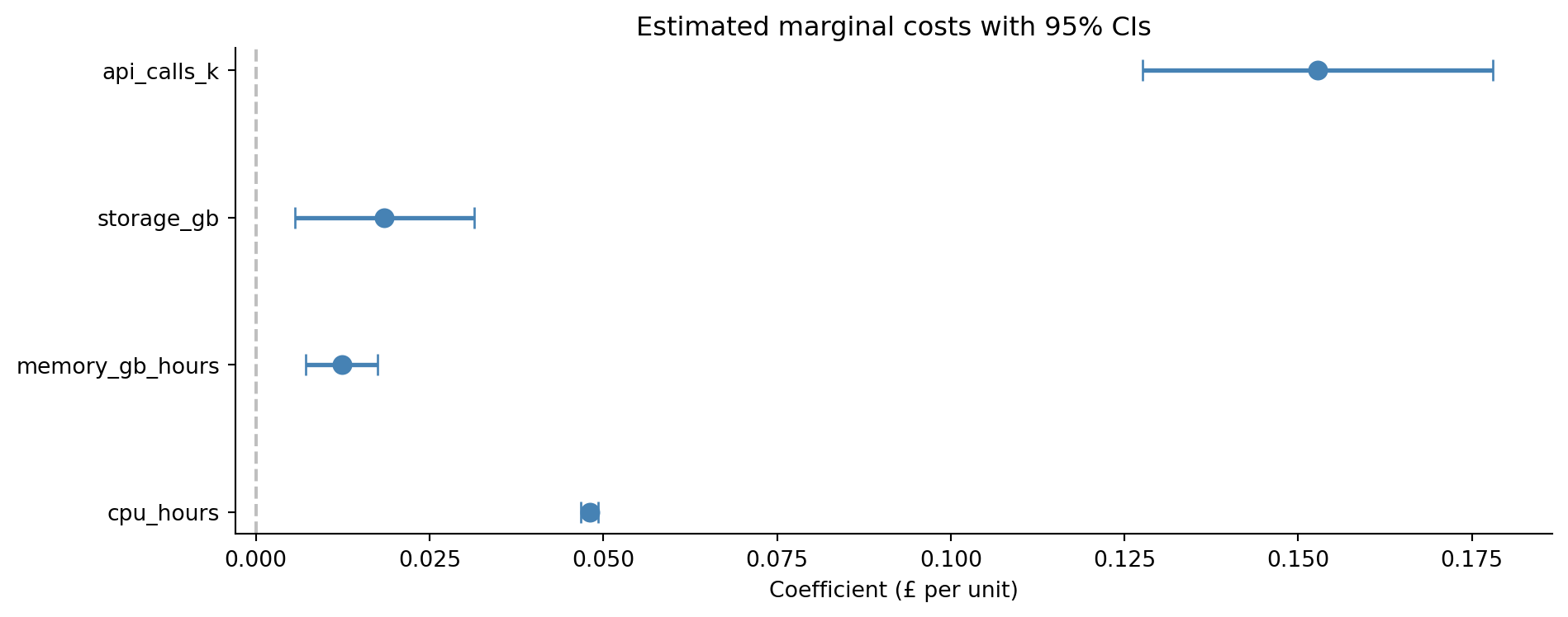
#| fig-cap: "Coefficient estimates with 95% confidence intervals. Each coefficient represents the marginal cost per unit of that resource, holding all other usage constant."
#| fig-alt: "Horizontal point-and-whisker chart showing four coefficient estimates with error bars. CPU hours, memory GB-hours, storage GB, and API calls per thousand each show a point estimate near their true value with narrow 95% confidence intervals, none of which cross zero."
coefs = cost_model.params[1:]  # skip intercept
ci = cost_model.conf_int().iloc[1:]

fig, ax = plt.subplots(figsize=(10, 4))
fig.patch.set_alpha(0)
ax.patch.set_alpha(0)
y_pos = range(len(feature_names))

ax.errorbar(coefs.values, y_pos,
            xerr=[coefs.values - ci.iloc[:, 0].values,
                  ci.iloc[:, 1].values - coefs.values],
            fmt='o', color='#0072B2', capsize=5, markersize=8, linewidth=2)

ax.set_yticks(list(y_pos))
ax.set_yticklabels(feature_names)
ax.set_xlabel('Coefficient (£ per unit)')
ax.set_title('Estimated marginal costs with 95% CIs')
ax.axvline(0, color='grey', linestyle='--', alpha=0.5)
ax.spines[['top', 'right']].set_visible(False)
plt.tight_layout()
plt.show()
```
The coefficient plot in @fig-coefficient-plot makes the results immediately actionable. CPU hours are the most expensive resource at £0.048 per hour, while memory costs £0.012 per GB-hour. But whether CPU or memory dominates a team's *total* bill depends on how much of each they consume: the coefficients tell you the rate, but the rate multiplied by the usage tells you the bill.
::: {.callout-tip}
## Author's Note
It's tempting to read coefficient magnitudes as importance rankings: a coefficient of 0.15 must matter more than one of 0.048. But that comparison is meaningless when the predictors have different units. A coefficient of 0.048 on CPU hours and 0.15 on API calls (in thousands) doesn't mean API calls are three times more important. One CPU hour costs £0.048; one *thousand* API calls cost £0.15; so one API call costs £0.00015, far cheaper than a CPU hour. The coefficient's magnitude depends entirely on the units of the predictor. If you want to compare relative importance, you need to standardise the predictors first (subtract the mean and divide by the standard deviation) so they're on a common scale. But don't always standardise; when you want interpretable units ("each CPU hour costs £0.048"), the raw coefficients are what you need. The choice between interpretability and comparability is a genuine trade-off, not a mistake to avoid.
:::
Here's what standardisation looks like in practice:
```{python}
#| label: standardised-coefficients
#| echo: true
# Standardise predictors to compare relative importance
X_std = (cloud_data[feature_names] - cloud_data[feature_names].mean()) / cloud_data[feature_names].std()
std_model = sm.OLS(y_cloud, sm.add_constant(X_std)).fit()

print('Standardised coefficients (effect of a 1 SD change in each predictor):')
for name in feature_names:
    print(f"  {name:20s}: £{std_model.params[name]:.2f}")
```
Now the coefficients are comparable: they each show the effect of a one-standard-deviation increase in that predictor. CPU hours dominate because they vary over a wide range *and* carry a meaningful per-unit cost.
## From inference to prediction {#sec-regression-prediction}
So far, we've used regression to *understand*: which predictors matter, what their effects are, and how confident we are about those effects. But regression also lets you *predict*. Given a new team's resource usage, what should their bill be?
This is where `scikit-learn` enters the picture. `statsmodels` is built for *inference*: it gives you p-values, confidence intervals, and diagnostic tests so you can understand *why* the model behaves the way it does. `scikit-learn` is built for *prediction*: it gives you a consistent fit/predict API optimised for evaluating how well the model generalises to new data. You'll often use both on the same problem: `statsmodels` to decide which predictors matter, then `scikit-learn` to build and evaluate the production model. This dual workflow carries through every model in Part 3.
```{python}
#| label: sklearn-prediction
#| echo: true
from sklearn.linear_model import LinearRegression
from sklearn.model_selection import train_test_split
from sklearn.metrics import root_mean_squared_error

# Split data: 80% for fitting (training), 20% for evaluation (testing)
X_features = cloud_data[feature_names]
y_target = cloud_data['monthly_cost']

X_train, X_test, y_train, y_test = train_test_split(
    X_features, y_target, test_size=0.2, random_state=42
)

# Fit on training data only (sklearn includes the intercept by default,
# unlike statsmodels which requires sm.add_constant)
lr = LinearRegression()
lr.fit(X_train, y_train)

# Evaluate on test data the model has never seen
y_pred = lr.predict(X_test)
rmse = root_mean_squared_error(y_test, y_pred)
r2_test = lr.score(X_test, y_test)  # .score() returns R² for LinearRegression

print(f"Coefficients:")
for name, coef in zip(feature_names, lr.coef_):
    print(f"  {name:20s}: £{coef:.4f} per unit")
print(f"  {'intercept':20s}: £{lr.intercept_:.2f}")

print(f"\nTest set performance:")
print(f"  RMSE: £{rmse:.2f}")
print(f"  R²:   {r2_test:.4f}")
```
The **train/test split** is a concept we haven't needed before, and it's fundamental to everything in Part 3. The idea is simple: fit the model on one subset of the data (the training set) and evaluate it on a separate subset (the test set) that the model has never seen. If the model only performs well on data it was trained on, it may be memorising noise rather than learning signal, the overfitting problem we flagged in @sec-dgp. The 80/20 split is conventional but not sacred; with fewer observations, you might want a larger training set, and later chapters will introduce cross-validation as a more principled alternative.
::: {.callout-note}
## Engineering Bridge
The train/test split is the ML equivalent of not running your tests against the same data you used to write them. Training data is your development environment; test data is production traffic. A model that only performs well on training data has passed its unit tests but fails against real-world inputs — it has overfit to the specifics of its training set rather than learning the underlying pattern. Just as you'd never ship code tested only against hand-picked inputs, you should never trust a model evaluated only on the data it was fitted to.
:::
**RMSE** (root mean squared error) is the square root of the average squared prediction error. It has the same units as $y$ (here, £), making it interpretable as a typical prediction error magnitude, though it weights large errors more heavily than small ones. For a model that satisfies its assumptions and includes all the relevant predictors, the RMSE on the test set should be close to the noise level $\sigma$ (the standard deviation of the noise term $\varepsilon$) in the data-generating process (here, £5).
```{python}
#| label: fig-predicted-vs-actual
#| echo: true
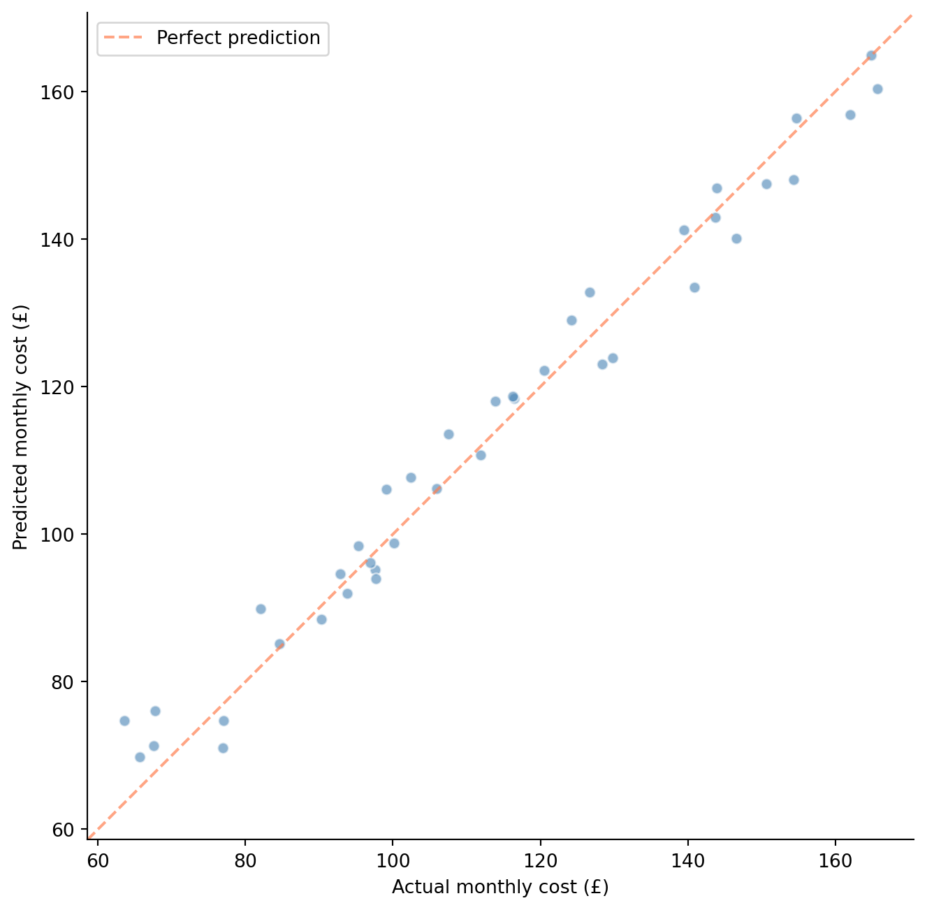
#| fig-cap: "Predicted vs actual monthly costs on the held-out test set. Points cluster tightly around the diagonal, indicating good predictive performance."
#| fig-alt: "Scatter plot of predicted monthly cost versus actual monthly cost for 40 test observations. Points cluster closely around a dashed orange diagonal line running from lower-left to upper-right, spanning roughly 60 to 180 pounds."
fig, ax = plt.subplots(figsize=(7, 7))
fig.patch.set_alpha(0)
ax.patch.set_alpha(0)
ax.scatter(y_test, y_pred, alpha=0.6, color='#0072B2', edgecolor='white')

# Perfect prediction line
lims = [min(y_test.min(), y_pred.min()) - 5,
        max(y_test.max(), y_pred.max()) + 5]
ax.plot(lims, lims, '#E69F00', linestyle='--', alpha=0.7, label='Perfect prediction')

ax.set_xlabel('Actual monthly cost (£)')
ax.set_ylabel('Predicted monthly cost (£)')
ax.set_xlim(lims)
ax.set_ylim(lims)
ax.set_aspect('equal')
ax.legend()
ax.spines[['top', 'right']].set_visible(False)
plt.tight_layout()
plt.show()
```
@fig-predicted-vs-actual shows predictions on unseen data clustering around the diagonal. You may notice the test $R^2$ is actually a touch *higher* than the training $R^2$ here. That ordering can feel wrong — we usually expect a model to look better on data it has already seen — but with only 40 test observations, sampling variability easily swamps the small generalisation gap, and this particular split happened to be slightly easier to predict. The lesson isn't that test performance beats training performance in general (it usually doesn't); it's that a single small split tells you very little, which is exactly why we lean on cross-validation. The gap becomes something to watch with more complex models. For a practical application, you could now predict costs for any new team:
```{python}
#| label: predict-new-team
#| echo: true
# Predict cost for a new team's usage
new_team = pd.DataFrame({
    'cpu_hours': [500],
    'memory_gb_hours': [200],
    'storage_gb': [50],
    'api_calls_k': [20],
})

predicted_cost = lr.predict(new_team)
print(f"Predicted monthly cost for new team: £{predicted_cost[0]:.2f}")
```
One thing to note: this prediction assumes the relationship between resources and costs stays stable. If your cloud provider changes pricing tiers or your teams adopt a new architecture that shifts usage patterns, the model's predictions will drift. You'd want to monitor prediction residuals over time, just as you'd monitor error rates after a deployment. If residuals start trending in one direction, it's time to retrain. We'll revisit this idea of model monitoring in Part 4.
You might also wonder about transforming or engineering the predictors before fitting. Common techniques include log-transforming skewed variables, creating **interaction terms** (new predictors formed by multiplying existing ones: does CPU cost more when memory is also high?), and encoding categorical predictors like cloud region into numerical form so the model can use them. These **feature engineering** choices are often where the real modelling skill lies, and we'll encounter them throughout Part 3.
## What can go wrong {#sec-regression-pitfalls}
Linear regression is robust and well understood, but it has failure modes you should recognise.
**Extrapolation.** The model knows nothing about the relationship outside the range of the training data. If your teams use between 100 and 2,000 CPU hours and you predict costs for a team using 10,000, you're assuming the linear relationship holds far beyond where you've observed it. Volume discounts, throttling, or tiered pricing could break that assumption entirely. Regression is an *interpolation* machine; extrapolation is a leap of faith.
**Multicollinearity.** When predictors are highly correlated with each other, the model struggles to separate their individual effects. If teams that use a lot of CPU also use a lot of memory (because they're running memory-intensive compute jobs), the model can't tell which resource is driving costs; it might assign an inflated coefficient to one and a deflated coefficient to the other, with both having large standard errors. The total prediction may still be accurate, but the individual coefficients become unreliable. Watch for unexpectedly large standard errors on predictors you'd expect to be significant. A diagnostic called the **variance inflation factor** (VIF) quantifies the problem: a VIF above 5 to 10 for a predictor signals that the *variance* of its coefficient estimate is substantially inflated by correlation with other predictors — the estimate becomes less precise, not systematically larger.
**Confounding and causation.** Regression coefficients describe associations, not causal effects. A **confounder** is a variable that influences both a predictor and the outcome, creating a spurious association between them. If teams that use more CPU also have more engineers, and you include CPU hours but not team size as a predictor, the CPU coefficient will absorb some of the team-size effect. The model predicts well, but interpreting the coefficient as "the cost of one more CPU hour" is misleading; it's partly picking up the effect of team size. This echoes the A/B testing insight from @sec-ab-testing: if you want causal claims, you need experimental design, not just statistical modelling.
**Influential observations.** A single unusual data point can pull the regression line substantially, especially if it has extreme predictor values (high **leverage**, meaning it sits far from the centre of the predictor space, giving it disproportionate pull on where the line falls). One team with 10× the typical CPU usage can dominate the slope estimate. Residual plots help here too: look for points that are both far from the trend *and* far from the centre of the data.
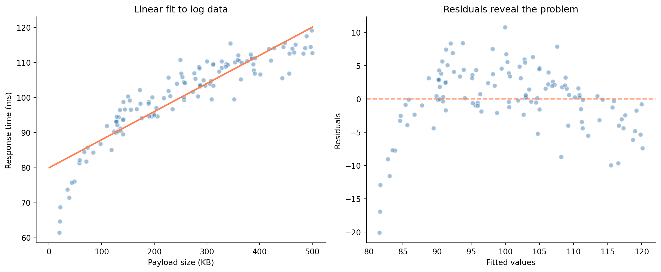
**Non-linearity.** If the true relationship curves, a straight line will systematically under-predict in some regions and over-predict in others. A systematic curve in the residuals vs fitted values (arch-shaped, as in the example below, or U-shaped, or S-shaped) signals a non-linear relationship the model is missing. The residual plots from @sec-residual-analysis are your first line of defence. For mild non-linearity, adding polynomial terms (like $x^2$) to your predictors can help. For more severe cases, the tree-based models we'll meet later in Part 3 handle non-linearity naturally.
To see what a failing model actually looks like, consider API response times that grow with request payload size, but with diminishing marginal cost per kilobyte (a log relationship, not a linear one):
```{python}
#| label: fig-failing-model
#| echo: true
#| fig-cap: "A linear model fit to non-linear data. Left: the fit looks reasonable at a glance. Right: the arch-shaped residual pattern reveals the model is systematically wrong — over-predicting at both extremes and under-predicting in the middle."
#| fig-alt: "Two-panel figure. Left: scatter plot of response time versus payload size with a straight regression line that misses the curve in the data. Right: residuals vs fitted values showing a clear arch-shaped pattern (positive in the middle, negative at the extremes), indicating model misspecification."
# Response time with a log relationship
rng_fail = np.random.default_rng(99)
payload_kb = rng_fail.uniform(1, 500, 120)
response_ms = 20 + 15 * np.log(payload_kb) + rng_fail.normal(0, 3, 120)

# Fit a linear model (wrong assumption)
X_payload = sm.add_constant(payload_kb)
wrong_model = sm.OLS(response_ms, X_payload).fit()

fig, (ax1, ax2) = plt.subplots(1, 2, figsize=(12, 5))
fig.patch.set_alpha(0)
ax1.patch.set_alpha(0)
ax2.patch.set_alpha(0)

# Data + fitted line
ax1.scatter(payload_kb, response_ms, alpha=0.5, color='#0072B2', edgecolor='white')
x_grid = np.linspace(1, 500, 200)
ax1.plot(x_grid, wrong_model.params[0] + wrong_model.params[1] * x_grid,
         '#E69F00', linewidth=2)
ax1.set_xlabel('Payload size (KB)')
ax1.set_ylabel('Response time (ms)')
ax1.set_title('Linear fit to log data')
ax1.spines[['top', 'right']].set_visible(False)

# Residuals — the arch shape is the diagnostic signal
ax2.scatter(wrong_model.fittedvalues, wrong_model.resid, alpha=0.5,
            color='#0072B2', edgecolor='white')
ax2.axhline(0, color='#E69F00', linestyle='--', alpha=0.7)
ax2.set_xlabel('Fitted values')
ax2.set_ylabel('Residuals')
ax2.set_title('Residuals reveal the problem')
ax2.spines[['top', 'right']].set_visible(False)

plt.tight_layout()
plt.show()
```
The scatter plot on the left might not immediately scream "wrong model"; the line looks plausible at a glance. But the residual plot on the right is unmistakable: that arch-shaped pattern tells you the model is systematically wrong. Log-transforming the predictor (`np.log(payload_kb)`) would fix it. This is why you always check residuals rather than relying on the fitted-line plot alone.
## Summary {#sec-linear-regression-summary}
1. **Linear regression models $y$ as a linear function of predictors** plus noise: $y = \beta_0 + \beta_1 x_1 + \cdots + \beta_p x_p + \varepsilon$. OLS finds the coefficients that minimise the sum of squared residuals.
2. **Each coefficient has a statistical interpretation** — its value, standard error, confidence interval, and p-value tell you the effect's size, precision, plausible range, and whether it's distinguishable from zero.
3. **Residual plots are your primary diagnostic tool.** Patterns in the residuals reveal violations of linearity, independence, normality, or equal variance — the model's hidden assumptions.
4. **In multiple regression, coefficients represent partial effects** — the change in $y$ per unit change in $x_j$, holding all other predictors constant. This is what makes regression more powerful than simple correlation.
5. **The train/test split separates fitting from evaluation.** A model that only works on data it's seen is useless. Evaluating on held-out data gives you an honest measure of predictive accuracy.
## Exercises {#sec-linear-regression-exercises}
1. Regenerate the pipeline duration data from this chapter (re-create `rng = np.random.default_rng(42)` and the same `files_changed` and `pipeline_duration` arrays). Then add a second predictor: `test_suites = np.clip(files_changed // 7 + rng.integers(0, 3, size=n), 1, 8)`. Fit a multiple regression and compare $R^2$ and adjusted $R^2$ to the simple regression. Does the second predictor improve the model? What do you notice about the coefficient standard errors?
2. Generate a dataset where the true relationship is quadratic ($y = 5 + 2x + 0.1x^2 + \varepsilon$) but fit a simple linear regression. Plot the residuals vs fitted values. What pattern reveals the model misspecification? Now add `x**2` as a second predictor and refit. How do the residual plots change?
3. **Multicollinearity exploration.** Generate two predictors that are highly correlated ($r > 0.95$) and both genuinely affect $y$. Fit a regression with both, then drop one and refit. How do the coefficient standard errors and p-values change? Calculate the variance inflation factor (VIF) using `statsmodels.stats.outliers_influence.variance_inflation_factor`.
4. **Conceptual:** Your team fits a regression predicting deployment failure rate from code churn, team size, and day of week. The coefficient for team size is negative — larger teams have fewer failures. A manager interprets this as "hiring more engineers reduces failures." Explain why this causal interpretation is problematic. What confounders might be at play?
5. Fit a linear regression on the scikit-learn `diabetes` dataset (`sklearn.datasets.load_diabetes()`). Perform the complete workflow: model fitting with `statsmodels` for inference, train/test evaluation with `scikit-learn`, and residual diagnostics. Which predictors are statistically significant? Does the model's $R^2$ on the test set match the training set?
6. **Conceptual:** It's natural to read a fitted regression as an invoice — each coefficient is the fixed "price per unit" of its predictor, and the prediction is the sum of the line items. Identify at least three situations from this chapter where that additive, independent-line-item reading breaks down, and say what each one does to the interpretation of a single coefficient.