---
# Content: CC BY-NC-SA 4.0 | Code: MIT - see /LICENSE.md
title: "Time series: modelling sequential data"
---
{{< include /_common-imports.qmd >}}
## When order matters {#sec-order-matters}
Every dataset we've worked with so far has been a collection of independent observations: rows in a table where shuffling the order wouldn't change the analysis. Scramble the 500 service telemetry records from @sec-too-many-features and every model we fitted would produce identical results. The rows were exchangeable.
Time series data is fundamentally different. The daily request count for your API gateway on Monday is not independent of Tuesday's count: if traffic spiked on Monday due to a product launch, it will probably remain elevated on Tuesday. A server's CPU utilisation at 14:00 is correlated with its utilisation at 13:59 in a way that it is not correlated with a random reading from last month. The *order* of observations carries information, and ignoring that order discards signal.
This is a familiar idea in engineering. Log streams, metric dashboards, deployment frequencies, error rate trends. Engineers work with sequential data constantly. The difference is that engineering tools typically *display* time series (Grafana dashboards, Datadog monitors) while data science tools *model* them: decomposing the series into interpretable components, quantifying the serial dependence between observations, and forecasting future values with calibrated uncertainty.
We'll work with a scenario that every platform engineer has encountered: capacity planning. Your team needs to forecast daily API request volumes to decide when to provision additional infrastructure, and the consequences of getting it wrong run in both directions. Over-provision and you waste money; under-provision and your service degrades under load.
```{python}
#| label: ts-data-setup
#| echo: true
#| code-fold: true
#| code-summary: "Expand to see API request volume simulation"
rng = np.random.default_rng(42)

# Simulate 3 years of daily API request volumes (in thousands)
n_days = 1095
dates = pd.date_range('2022-01-01', periods=n_days, freq='D')

# Components of the series
day_of_year = np.arange(n_days) % 365.25  # 365.25 approximates leap-year drift

# Trend: gradual growth from organic adoption (~100k to ~250k daily requests)
trend = 100 + 150 * (np.arange(n_days) / n_days) ** 0.8

# Seasonality: weekly cycle (lower on weekends) + annual cycle (peak in summer, trough in winter/January)
weekly = -12 * np.isin(dates.dayofweek, [5, 6]).astype(float)
annual = -15 * np.cos(2 * np.pi * day_of_year / 365.25) + 8 * np.sin(4 * np.pi * day_of_year / 365.25)

# Noise: autocorrelated residuals (today's noise influences tomorrow's)
noise = np.zeros(n_days)
for t in range(1, n_days):
    noise[t] = 0.4 * noise[t - 1] + rng.normal(0, 8)

requests = trend + weekly + annual + noise
requests = np.maximum(requests, 10)  # floor at 10k

ts = pd.DataFrame({'date': dates, 'requests_k': requests})
ts = ts.set_index('date')
ts = ts.asfreq('D')
```
```{python}
#| label: fig-ts-overview
#| echo: true
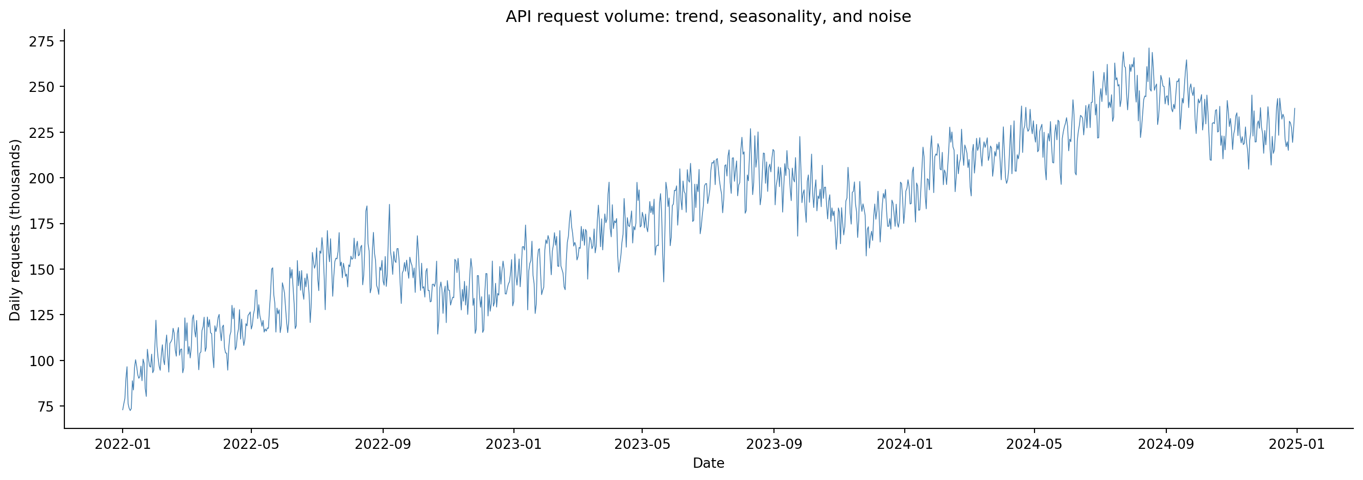
#| fig-cap: "Three years of daily API request volume (thousands). The series shows a clear upward trend, weekly seasonality (weekend dips), and irregular fluctuations around the pattern."
#| fig-alt: "Line chart of daily API request volume from January 2022 to December 2024. The series rises from roughly 100 to 250 thousand requests per day with a visible upward trend. Regular weekly dips are visible as a sawtooth pattern, and broader annual seasonality creates gentle waves. Random day-to-day variation adds noise throughout."
fig, ax = plt.subplots(figsize=(14, 5))
fig.patch.set_alpha(0)
ax.patch.set_alpha(0)
ax.plot(ts.index, ts['requests_k'], linewidth=0.6, color='#0072B2')
ax.set_xlabel('Date')
ax.set_ylabel('Daily requests (thousands)')
ax.set_title('API request volume: trend, seasonality, and noise')
ax.spines[['top', 'right']].set_visible(False)
plt.tight_layout()
plt.show()
```
Even at a glance, @fig-ts-overview reveals structure. There's an upward **trend** as the platform grows. There are regular dips: the weekly pattern of lower weekend traffic. And there's irregular day-to-day variation that no deterministic pattern can explain. Time series analysis gives us tools to decompose, quantify, and forecast these components.
## Decomposition: trend, seasonality, and residuals {#sec-decomposition}
The standard way to think about a time series is as the sum (or product) of three components:
$$
y_t = T_t + S_t + R_t
$$
where $y_t$ is the observed value at time $t$, $T_t$ is the **trend** (the long-run direction), $S_t$ is the **seasonal** component (repeating patterns at fixed intervals), and $R_t$ is the **residual** (everything left over, the noise). This additive decomposition assumes the seasonal swings stay roughly constant in absolute size as the trend changes. When seasonal amplitude grows proportionally with the level (common in financial data), a multiplicative decomposition ($y_t = T_t \times S_t \times R_t$) is more appropriate.
The `statsmodels` library provides `seasonal_decompose`, which estimates these components using moving averages. It's a useful exploratory tool, though it can only handle a single seasonal period at a time. More sophisticated methods like STL (Seasonal and Trend decomposition using Loess) handle outliers more robustly and allow the seasonal component to evolve over time.
```{python}
#| label: fig-decomposition
#| echo: true
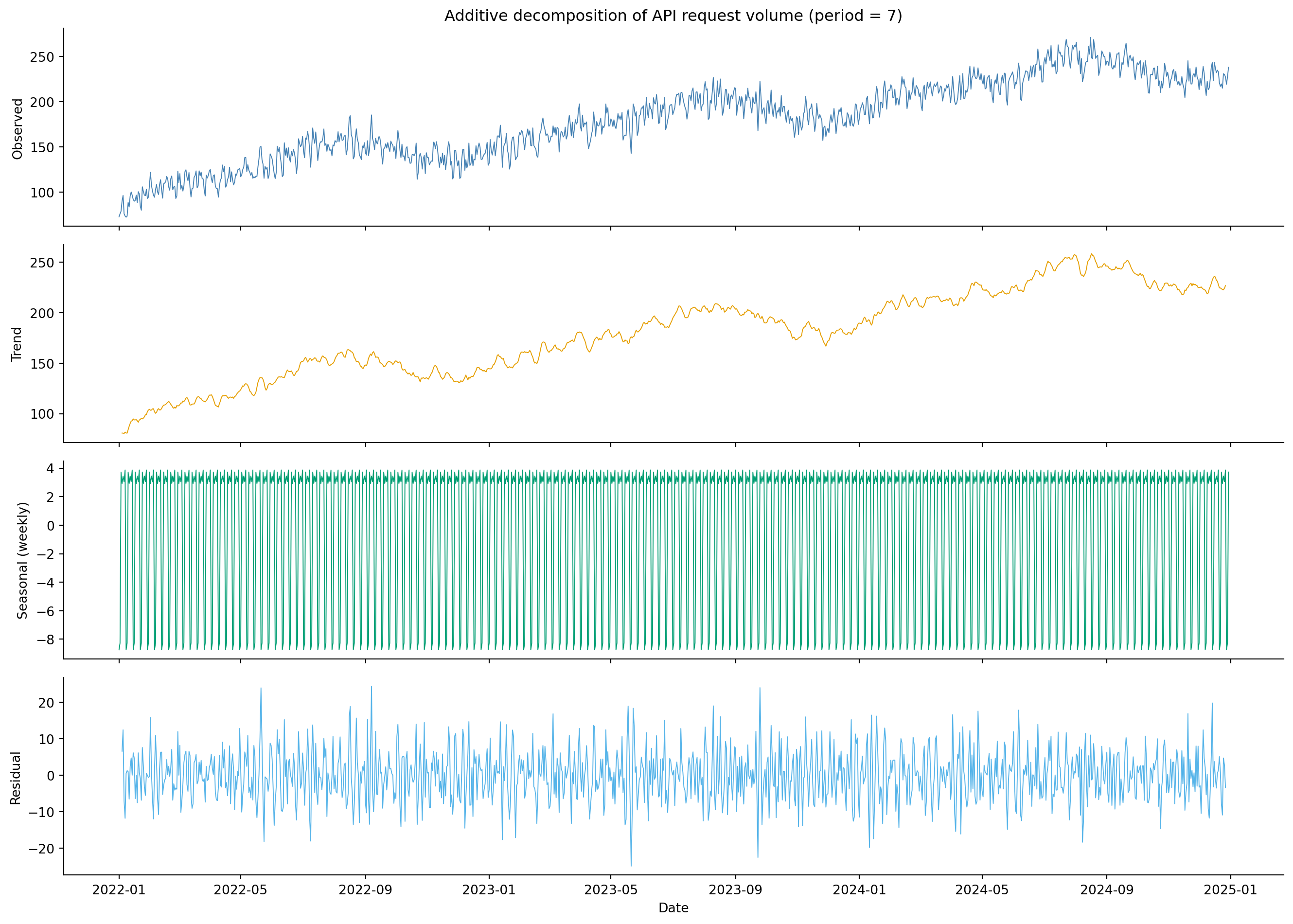
#| fig-cap: "Additive decomposition of the API request series with `period=7`. The trend captures both gradual growth and the slower annual cycle (the 7-day smoothing window is too short to separate them), the seasonal component reveals the weekly traffic cycle (weekend dips), and the residuals are close to white noise."
#| fig-alt: "Four-panel stacked figure showing the additive decomposition of the API request time series. Top panel: the raw observed series rising from 100 to 250 with visible oscillations. Second panel: an upward trend line carrying broad annual undulations on top of the growth. Third panel: a repeating weekly pattern oscillating around zero with regular dips. Bottom panel: residuals scattered randomly around zero with no obvious trend or cycle."
from statsmodels.tsa.seasonal import seasonal_decompose

decomposition = seasonal_decompose(ts['requests_k'], model='additive', period=7)

fig, axes = plt.subplots(4, 1, figsize=(14, 10), sharex=True)
fig.patch.set_alpha(0)
components = [
    (decomposition.observed, 'Observed', '#0072B2'),
    (decomposition.trend, 'Trend', '#E69F00'),
    (decomposition.seasonal, 'Seasonal (weekly)', '#009E73'),
    (decomposition.resid, 'Residual', '#666666'),
]

for ax, (data, label, colour) in zip(axes, components):
    ax.patch.set_alpha(0)
    ax.plot(data, linewidth=0.7, color=colour)
    ax.set_ylabel(label)
    ax.spines[['top', 'right']].set_visible(False)

axes[-1].set_xlabel('Date')
axes[0].set_title('Additive decomposition of API request volume (period = 7)')
plt.tight_layout()
plt.show()
```
As @fig-decomposition shows, the decomposition confirms what we saw visually. The trend component shows steady growth. The seasonal component captures the weekly rhythm of lower weekend traffic (with `period=7`). Notice that because `seasonal_decompose` handles only one period at a time, the annual seasonality — the broader waves visible in the raw series — is absorbed into the trend component, because the trend is a 7-day moving average wide enough to track the slow annual wave; a clean separation needs a method like STL with two seasonal periods. If the residuals show clear low-frequency patterns, that's a sign the decomposition has missed a seasonal component. Exercise 1 explores what happens when you decompose with `period=365` instead.
::: {.callout-note}
## Engineering Bridge
Decomposition is **separation of concerns** applied to data. Just as you decompose a monolithic service into independent components (authentication, business logic, data access) to reason about each in isolation, time series decomposition separates a complex signal into trend (the long-term architecture), seasonality (the predictable traffic pattern), and residuals (the unpredictable noise). Each component can be analysed, modelled, and monitored independently. Where the analogy breaks down: service components interact through defined interfaces, while time series components are statistically estimated and may bleed into each other: the boundary between "trend" and "low-frequency seasonality" is not always sharp.
:::
## Stationarity: the assumption everything rests on {#sec-stationarity}
Most time series models assume the series is **stationary**: that its statistical properties (mean, variance, autocorrelation structure) don't change over time. A stationary series fluctuates around a constant level with constant variability. Our raw API request series is clearly not stationary: it has an upward trend, so the mean is rising.
Why does stationarity matter? Because models learn patterns from historical data and apply them to the future. If the mean is rising, a model trained on last year's data will systematically underpredict this year's values. Stationarity ensures that patterns observed in the past remain relevant in the future. Think of it as the assumption behind your monitoring baselines: if the system's behaviour changes fundamentally (an architecture migration, a new dependency), the baselines you learned from last month's data become misleading. Non-stationarity in a time series is the same problem: the statistical properties the model learned from the past no longer describe the present.
The standard diagnostic is the **Augmented Dickey-Fuller** (ADF) test, which tests the null hypothesis that the series has a **unit root**, a specific form of non-stationarity where shocks persist indefinitely rather than decaying. Rejecting the null (a low p-value) provides evidence against the unit root, suggesting the series is stationary. Failing to reject (a high p-value) means the data is consistent with a unit root, though this could also reflect limited statistical power rather than genuine non-stationarity.
```{python}
#| label: stationarity-test
#| echo: true
from statsmodels.tsa.stattools import adfuller

def adf_report(series, name):
    result = adfuller(series.dropna(), autolag='AIC')
    stat, pval = result[0], result[1]
    conclusion = 'reject unit root (stationary)' if pval < 0.05 else 'fail to reject unit root (non-stationary)'
    print(f"  {name:25s}  ADF={stat:7.3f}  p={pval:.4f}  → {conclusion}")

print('Augmented Dickey-Fuller test results:')
adf_report(ts['requests_k'], 'Raw series')

# First difference: y_t - y_{t-1}
ts['diff'] = ts['requests_k'].diff()
adf_report(ts['diff'], 'First difference')
```
The raw series fails the stationarity test (high p-value: we cannot reject the unit root), but **differencing**, computing the change from one day to the next ($\Delta y_t = y_t - y_{t-1}$), removes most of the trend and yields a series the ADF test treats as stationary. (Real trends are rarely exactly linear, so differencing is an approximation rather than a perfect remedy.) This is the standard remedy: if the series has a trend, difference it. If it has seasonal non-stationarity, apply a seasonal difference ($y_t - y_{t-s}$ where $s$ is the season length). The number of differences required is called the **order of integration**: a series that needs one difference to become stationary is called **integrated of order 1**, or $I(1)$.
## Autocorrelation: the memory of a time series {#sec-autocorrelation}
In a stationary time series, the key structure is **autocorrelation**: the correlation between the series and lagged versions of itself. If today's API traffic is high, how much does that tell us about tomorrow's traffic? About next week's?
The **autocorrelation function** (ACF) measures the correlation between $y_t$ and $y_{t-k}$ for each lag $k$. The **partial autocorrelation function** (PACF) measures the correlation between $y_t$ and $y_{t-k}$ after removing the effect of all intermediate lags ($y_{t-1}, y_{t-2}, \ldots, y_{t-k+1}$). The distinction matters because correlation can propagate through a chain: if today correlates with tomorrow and tomorrow with the day after, today will appear correlated with the day after even if there's no direct relationship. The PACF strips out this indirect correlation.
```{python}
#| label: fig-acf-pacf
#| echo: true
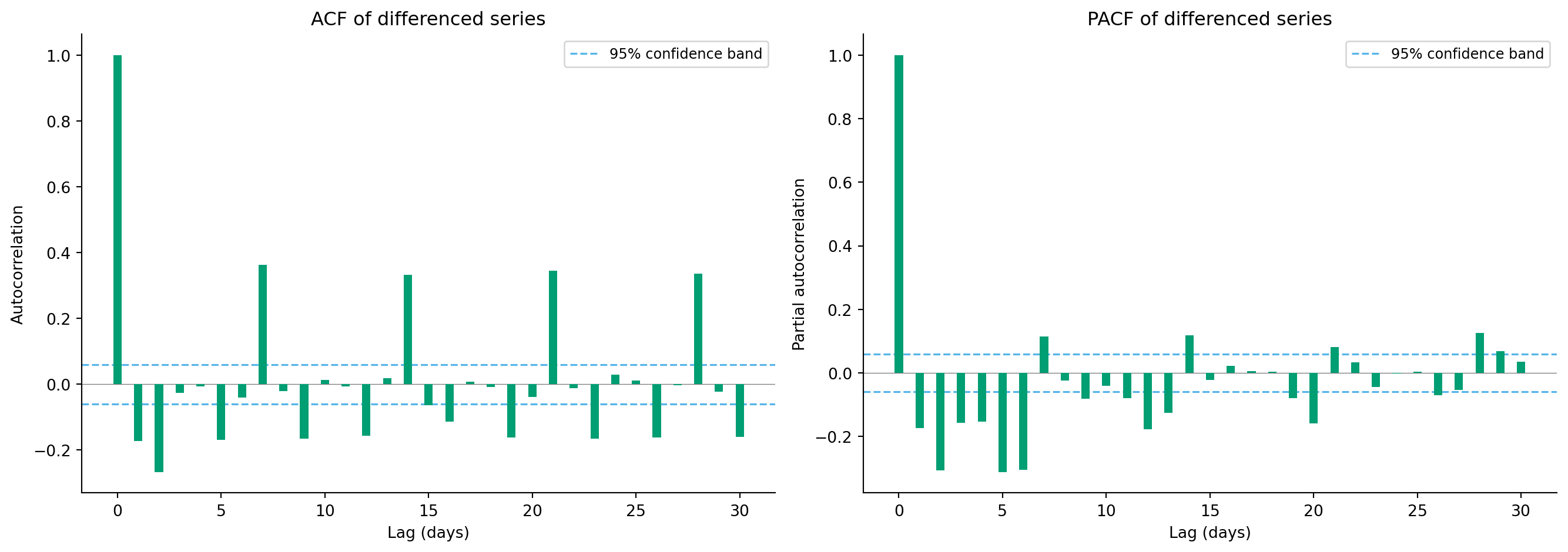
#| fig-cap: "ACF and PACF of the differenced API request series. The ACF shows significant correlation at lag 7 (weekly pattern) and its multiples. The PACF shows a negative spike at lag 1 (today's change partially reverses yesterday's) and significant structure at lag 7."
#| fig-alt: "Two-panel figure. Left: bar chart of autocorrelation values at lags 0 to 30 for the differenced series, with green bars. A notable spike appears at lag 7 and smaller spikes at lags 14 and 21, indicating a weekly cycle. Dashed horizontal lines mark the 95 percent confidence bands. Most lags between the weekly spikes fall within the bands. Right: partial autocorrelation bar chart with green bars showing a negative spike at lag 1, and significant spikes at lag 7. Dashed confidence bands are shown in the same style."
from statsmodels.tsa.stattools import acf, pacf

diff = ts['diff'].dropna()
n_obs = len(diff)
acf_vals = acf(diff, nlags=30, fft=True)
pacf_vals = pacf(diff, nlags=30, method='ywm')

# 95% confidence band: approximate ±1.96 / sqrt(n)
conf = 1.96 / np.sqrt(n_obs)

fig, (ax1, ax2) = plt.subplots(1, 2, figsize=(14, 5))
fig.patch.set_alpha(0)

for ax, vals, title, ylabel in [
    (ax1, acf_vals, 'ACF of differenced series', 'Autocorrelation'),
    (ax2, pacf_vals, 'PACF of differenced series', 'Partial autocorrelation'),
]:
    ax.patch.set_alpha(0)
    # Start from lag 1 to omit the uninformative lag-0 spike (always 1.0)
    lags = np.arange(1, len(vals))
    ax.bar(lags, vals[1:], width=0.4, color='#009E73', edgecolor='none', zorder=3)
    ax.axhline(conf, color='#56B4E9', linestyle='--', linewidth=1.2,
               label='95% confidence band')
    ax.axhline(-conf, color='#56B4E9', linestyle='--', linewidth=1.2)
    ax.axhline(0, color='grey', linewidth=0.5)
    ax.set_title(title)
    ax.set_xlabel('Lag (days)')
    ax.set_ylabel(ylabel)
    ax.legend(loc='upper right', fontsize=9)
    ax.spines[['top', 'right']].set_visible(False)

plt.tight_layout()
plt.show()
```
The ACF and PACF plots (@fig-acf-pacf) are the primary diagnostic tools for identifying time series structure. The significant spike at lag 7 in the ACF confirms the weekly seasonality. The negative spike at lag 1 in the PACF tells us that today's change tends to partially reverse yesterday's, a common pattern in differenced series where the noise has short-term persistence. These patterns guide model selection: the weekly spikes suggest seasonal terms with period 7, and the lag-1 structure suggests at least one AR or MA term.
::: {.callout-note}
## Engineering Bridge
Autocorrelation is the statistical formalisation of something engineers already monitor: **metric persistence**. When your CPU utilisation spikes, you don't expect it to return to baseline instantly; high load tends to persist for a while before subsiding. That persistence *is* positive autocorrelation at short lags. The ACF plot quantifies exactly how long the "memory" of a spike lasts and how strong it is at each interval. If you've ever tuned an alerting system's smoothing window, set a cooldown period for autoscaling rules, or configured a burn rate for an error budget, you were implicitly reasoning about autocorrelation structure. A 5-minute smoothing window assumes that meaningful signal persists across at least 5 minutes of observations. That's an assertion about the autocorrelation at short lags being high enough to warrant averaging.
:::
## ARIMA: the workhorse model {#sec-arima}
**ARIMA** (AutoRegressive Integrated Moving Average) is the classical framework for time series forecasting, formalised by Box and Jenkins [@boxjenkins1976]. The name describes its three ingredients, each controlled by a parameter. The autoregressive (AR) component models each value as a linear function of its own recent past: how strongly yesterday's traffic predicts today's, and how far back that dependence extends. The parameter $p$ controls how many past values to include; an AR(2) model, for instance, uses the previous two values. The "integrated" part handles non-stationarity: rather than modelling the raw series, ARIMA works on the differenced series, with $d$ specifying how many rounds of differencing are needed (typically 0 or 1). The moving average (MA) component captures the influence of past forecast errors: if yesterday's prediction overshot by 5k requests, part of today's prediction should account for that overshoot. The parameter $q$ controls how many past errors are included.
Together, an ARIMA($p, d, q$) model combines all three. The differencing operator $\Delta$ subtracts each value from the previous one ($\Delta y_t = y_t - y_{t-1}$), and $\Delta^d$ means applying it $d$ times. For the differenced series $w_t = \Delta^d y_t$:
$$
w_t = \phi_1 w_{t-1} + \cdots + \phi_p w_{t-p} + \varepsilon_t + \theta_1 \varepsilon_{t-1} + \cdots + \theta_q \varepsilon_{t-q}
$$
where $\phi_1, \ldots, \phi_p$ are the AR coefficients (how much each past value contributes), $\theta_1, \ldots, \theta_q$ are the MA coefficients (how much each past error contributes), and $\varepsilon_t$ is *white noise*: random, uncorrelated errors with zero mean and constant variance. In plain English: today's value equals a weighted combination of recent values, plus a weighted combination of recent forecast errors, plus a fresh random shock. When differencing is applied ($d \geq 1$), including a constant introduces a deterministic drift, a linear trend in the original series levels, which is often undesirable. When $d = 0$, the constant captures the mean of the stationary series.
To handle seasonality, we extend to **SARIMA** (Seasonal ARIMA), which adds seasonal AR, differencing, and MA terms with period $s$. A SARIMA model is written as ARIMA($p, d, q$)($P, D, Q$)$_s$, where $P$, $D$, $Q$ are the seasonal counterparts and $s$ is the season length. The seasonal terms operate at multiples of $s$: for weekly data ($s = 7$), a seasonal AR(1) term captures how this Monday relates to last Monday.
::: {.callout-tip}
## Author's Note
ARIMA notation looks dense, but it is actually a compact configuration string. Once you decompose it, ARIMA(1,1,1)(1,1,1)$_7$ reads as clearly as a JSON config: one AR lag, one difference, one MA lag, plus the same seasonal structure at a weekly period. Think of it as `ARIMA(p=1, d=1, q=1, P=1, D=1, Q=1, s=7)`. Seven integers fully define the model's structure. The density is the feature, not the bug: a single compact expression fully specifies a model that would take a paragraph to describe in prose.
:::
Rather than manually choosing $p$, $d$, $q$ and their seasonal counterparts through ACF/PACF analysis alone, you can compare models systematically using information criteria like AIC (Akaike Information Criterion). AIC balances model fit against complexity, the same bias-variance trade-off from @sec-bias-variance, expressed as a single number. Lower AIC is better. The `statsmodels` library supports fitting SARIMA models directly; `pmdarima` (a separate package, not included in this book's dependencies) provides an `auto_arima` function that automates the search over parameter combinations.
```{python}
#| label: arima-fit
#| echo: true
from statsmodels.tsa.statespace.sarimax import SARIMAX

# Hold out the last 90 days for evaluation
train = ts['requests_k'][:-90]
test = ts['requests_k'][-90:]

# Fit SARIMA(1,1,1)(1,1,1)_7 — a reasonable starting point given the ACF/PACF
# enforce_stationarity/invertibility=False allows the optimiser to explore
# parameter values near the boundary of the stationarity/invertibility regions,
# which sometimes helps numerical convergence
model = SARIMAX(train, order=(1, 1, 1), seasonal_order=(1, 1, 1, 7),
                enforce_stationarity=False, enforce_invertibility=False)
fit = model.fit(disp=False)

print(fit.summary().tables[1])
print(f"\nAIC: {fit.aic:.1f}")
```
## Model diagnostics {#sec-ts-diagnostics}
Before trusting a forecast, check whether the model has captured the series structure adequately. The residuals from a well-fitted model should resemble white noise: no remaining autocorrelation, roughly constant variance, and approximately normal distribution. Patterned residuals indicate that the model has missed structure that could improve forecasts.
```{python}
#| label: fig-residual-diagnostics
#| echo: true
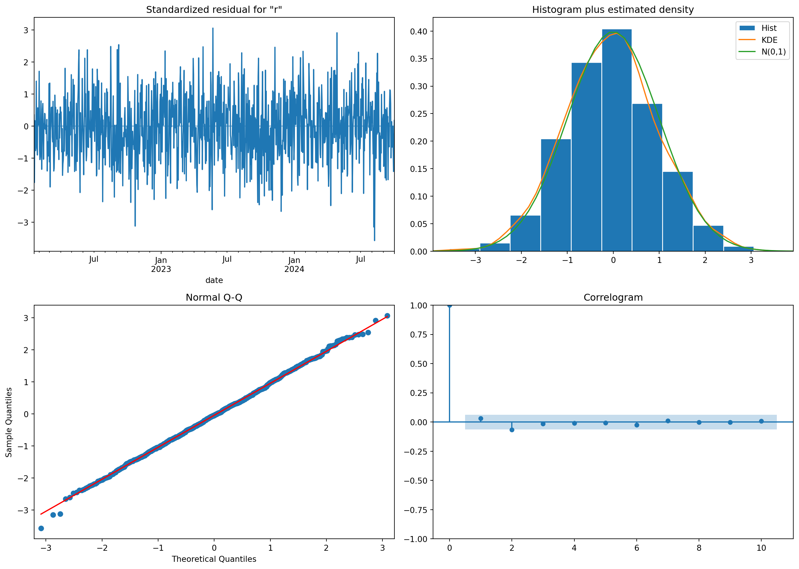
#| fig-cap: "Residual diagnostics for the SARIMA model. Top left: standardised residuals over time (no visible pattern). Top right: histogram of residuals with a normal density overlay. Bottom left: Q-Q plot checking normality. Bottom right: correlogram of residuals (no significant autocorrelation remaining)."
#| fig-alt: "Four-panel diagnostic figure. First panel: standardised residuals scattered around zero with no visible trend. Second panel: histogram of residuals closely following a normal curve with slightly heavier tails. Third panel: Q-Q plot where points track the diagonal through middle quantiles with mild deviation at extremes. Fourth panel: correlogram of residuals with all bars within the confidence band, confirming no remaining autocorrelation."
fig = fit.plot_diagnostics(figsize=(14, 10))
fig.patch.set_alpha(0)
for ax in fig.get_axes():
    ax.patch.set_alpha(0)
plt.tight_layout()
plt.show()
```
The four panels in @fig-residual-diagnostics check complementary aspects of model adequacy. The standardised residuals plot should show no trends, clusters of volatility, or other patterns, just random scatter around zero. The histogram and Q-Q plot test whether residuals are approximately normal, which affects the validity of prediction intervals (mild departures from normality are common and usually acceptable). The correlogram checks for remaining autocorrelation; any significant spikes suggest the model has missed a lag relationship that could be captured by adjusting $p$, $q$, or the seasonal parameters.
## Forecasting with uncertainty {#sec-forecasting}
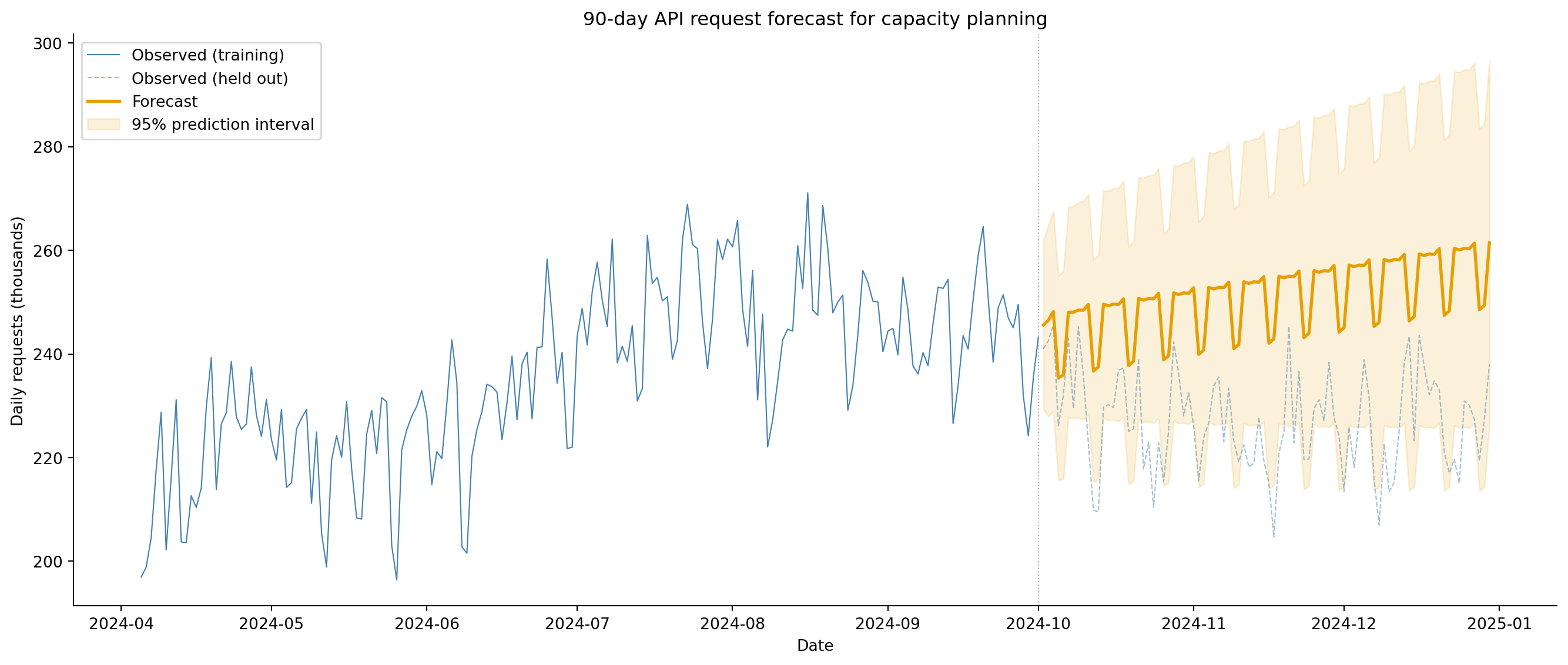
The practical goal of time series modelling is forecasting: predicting future values with calibrated uncertainty. SARIMA produces both a point forecast (the expected value) and a prediction interval (the range of plausible outcomes). For capacity planning, both matter: the point forecast guides your default provisioning, and the upper bound of the interval defines the headroom you need to avoid service degradation.
```{python}
#| label: fig-forecast
#| echo: true
#| fig-cap: "90-day forecast with 95% prediction intervals. The forecast captures the upward trend and weekly seasonality. The prediction interval widens as the horizon extends — uncertainty grows the further you predict into the future."
#| fig-alt: "Line chart with four visual elements. A solid line shows the last 180 days of observed training data rising from about 210 to 240 thousand requests. A dashed line shows the 90 held-out actual values continuing the upward trend with weekly oscillations. A solid forecast line tracks the upward trend and weekly dips. A shaded region around the forecast shows the 95 percent prediction interval, starting narrow at the forecast origin and widening progressively to about plus or minus 30 thousand by day 90, reflecting increasing uncertainty over the forecast horizon."
# Generate forecast with prediction intervals
forecast = fit.get_forecast(steps=90)
forecast_mean = forecast.predicted_mean
confidence = forecast.conf_int(alpha=0.05)

fig, ax = plt.subplots(figsize=(14, 6))
fig.patch.set_alpha(0)
ax.patch.set_alpha(0)

# Plot last 180 days of training data for context
recent = train[-180:]
ax.plot(recent.index, recent, color='#0072B2', linewidth=0.8,
        label='Observed (training)')
ax.plot(test.index, test, color='#CC79A7', linewidth=1.5,
        linestyle='--', label='Observed (held out)')

# Forecast
ax.plot(forecast_mean.index, forecast_mean, color='#E69F00', linewidth=2,
        label='Forecast')
ax.fill_between(confidence.index,
                confidence.iloc[:, 0], confidence.iloc[:, 1],
                color='#E69F00', alpha=0.15, label='95% prediction interval')

# Boundary between training and forecast
ax.axvline(train.index[-1], color='grey', linestyle=':', linewidth=0.8,
           alpha=0.6)

ax.set_xlabel('Date')
ax.set_ylabel('Daily requests (thousands)')
ax.set_title('90-day API request forecast for capacity planning')
ax.legend(loc='upper left')
ax.spines[['top', 'right']].set_visible(False)
plt.tight_layout()
plt.show()
```
The widening prediction interval in @fig-forecast is a feature, not a defect. It honestly communicates that forecasts become less certain as the horizon extends, a point that dashboards showing only a single forecast line often obscure. For capacity planning, the *upper bound* of the prediction interval matters more than the point forecast: you need enough infrastructure to handle the plausible worst case, not just the expected case.
```{python}
#| label: forecast-evaluation
#| echo: true
from sklearn.metrics import mean_absolute_error, root_mean_squared_error

# Naive baseline: repeat the final training week (seasonal naive)
naive = np.tile(train.values[-7:], 13)[:len(test)]
naive_mae = mean_absolute_error(test, naive)

# SARIMA evaluation against held-out data
mae = mean_absolute_error(test, forecast_mean)
rmse = root_mean_squared_error(test, forecast_mean)
coverage = ((test >= confidence.iloc[:, 0]) &
            (test <= confidence.iloc[:, 1])).mean()

print('Forecast evaluation (90-day horizon):')
print(f"  Naive MAE (repeat last week):  {naive_mae:.1f}k requests")
print(f"  SARIMA MAE:                    {mae:.1f}k requests")
print(f"  SARIMA RMSE:                   {rmse:.1f}k requests")
print(f"  95% interval coverage:         {coverage:.1%}")
```
The naive baseline, simply repeating the last observed week, provides an important sanity check. If SARIMA can't beat this trivial forecast, the additional modelling complexity isn't earning its keep. The **coverage** metric is especially important: if the 95% prediction interval actually contains about 95% of the held-out observations, the model's uncertainty estimates are well-calibrated. Coverage well below 95% means the intervals are too narrow (the model is overconfident); well above 95% means they're too wide.
Note that our SARIMA model only captures weekly seasonality ($s = 7$). The underlying data also contains an annual cycle (see the data-generation code), which the model doesn't explicitly account for. If coverage falls notably below 95%, the unmodelled annual component is a likely culprit: the residual variance estimate doesn't include this systematic pattern, leading to intervals that are too narrow. A more complete approach would add annual seasonality via Fourier features in a SARIMAX model or use a method like Prophet that handles multiple seasonal periods natively.
::: {.callout-note}
## Engineering Bridge
Prediction interval coverage is the time series analogue of **SLO compliance**. An SLO says "99.9% of requests complete in under 300ms" — if you measure 99.5%, your SLO is breached. A 95% prediction interval says "95% of future observations should fall within this range" — if only 80% do, your model is miscalibrated. In both cases, you're comparing a *claimed* probability against *observed* frequency. The monitoring infrastructure is the same: track the hit rate over a rolling window and alert when it drifts. An error budget for your forecast model is just as valuable as one for your production service.
:::
## The train-test split for time series {#sec-ts-validation}
A critical difference from cross-sectional data: you cannot randomly split time series data into training and test sets. Random splitting would leak future information into the training set: the model could learn patterns from December data to predict October values, which it would never have access to in real forecasting. The split must respect temporal order: train on the past, test on the future.
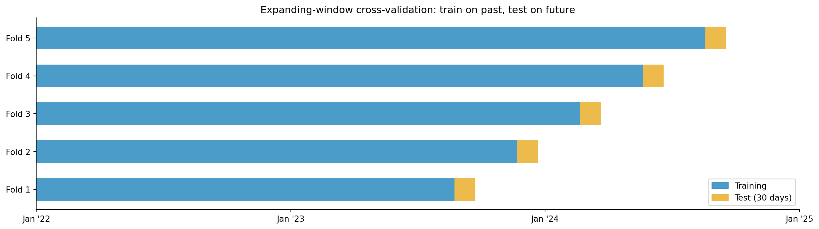
The approach we used (training on all data except the last 90 days and evaluating on those held-out days) is the simplest valid strategy. For more robust evaluation, **expanding-window cross-validation** trains on all data up to a split point and forecasts a fixed horizon ahead, repeating with the split point advancing through the series. (The closely related **rolling-window** variant keeps a fixed-size training window that slides forward, discarding early observations. In practice, expanding-window is more common because discarding early data wastes information.)
```{python}
#| label: fig-expanding-cv
#| echo: true
#| fig-cap: "Expanding-window cross-validation for time series. Each fold trains on all data up to the split point and forecasts the next 30 days. Successive folds include more training data, simulating the real forecasting task and producing multiple independent error estimates."
#| fig-alt: "Schematic diagram showing five horizontal bars stacked vertically, each representing a cross-validation fold. In each bar, the left portion (training) grows longer from top to bottom, and the right portion (test, 30 days) stays fixed in width but shifts forward in time. The x-axis is labelled with year markers from January 2022 to January 2025. A legend identifies training and test regions."
fig, ax = plt.subplots(figsize=(14, 4))
fig.patch.set_alpha(0)
ax.patch.set_alpha(0)

n_folds = 5
fold_test_size = 30
fold_gap = 90

for i in range(n_folds):
    train_end = 600 + i * fold_gap
    test_end = train_end + fold_test_size

    ax.barh(i, train_end, left=0, height=0.6, color='#0072B2',
            alpha=0.7, edgecolor='none')
    ax.barh(i, fold_test_size, left=train_end, height=0.6, color='#E69F00',
            alpha=0.7, edgecolor='none')

ax.set_yticks(range(n_folds))
ax.set_yticklabels([f'Fold {i+1}' for i in range(n_folds)])
ax.set_xticks([0, 365, 730, 1095])
ax.set_xticklabels(["Jan '22", "Jan '23", "Jan '24", "Jan '25"])
ax.set_xlim(0, 1095)
ax.set_title('Expanding-window cross-validation: train on past, test on future')

# Manual legend
from matplotlib.patches import Patch
ax.legend(handles=[Patch(color='#0072B2', alpha=0.7, label='Training'),
                   Patch(color='#E69F00', alpha=0.7, label='Test (30 days)')],
          loc='lower right')
ax.spines[['top', 'right']].set_visible(False)
plt.tight_layout()
plt.show()
```
This expanding-window approach (@fig-expanding-cv) is essential because time series models can appear accurate on a single split while failing on others; perhaps the held-out period happened to be unusually predictable or fell during a stable phase. Multiple splits give a more honest picture of forecast performance and reveal whether accuracy degrades as the series evolves.
::: {.callout-tip}
## Author's Note
The train-test split for time series is where habits from supervised learning become actively dangerous. The instinct to reach for `train_test_split` with `shuffle=True` is strong: it's the right thing to do for cross-sectional data. But with time series, random shuffling lets the model "see the future," and the results look spectacular, but suspiciously good. The rule is simple: always split *in time*, never randomly. This is one of the few places in data science where a single conceptual mistake, forgetting that order matters, can completely invalidate your results. If your time series model looks too good to be true, the first thing to check is whether information from the future leaked into the training set.
:::
## Beyond ARIMA {#sec-beyond-arima}
ARIMA is the classical workhorse, but it has limitations. It assumes linear relationships between lagged values, it handles only a single seasonal period well (our weekly cycle), and parameter selection can be finicky. Several modern alternatives address these limitations, and the choice between them depends on the structure of your data and your operational priorities.
**Exponential smoothing**, the ETS (Error, Trend, Seasonal) family, is a complementary classical approach that models trend and seasonality through weighted averages of past observations, with more recent observations weighted more heavily. Where ARIMA works with the autocorrelation structure of the differenced series, ETS directly models the level, trend, and seasonal components and updates them as new observations arrive. ETS is often competitive with ARIMA for univariate forecasting and can be easier to interpret, since each component has a direct physical meaning. The `statsmodels` `ExponentialSmoothing` class implements the main variants.
Prophet, developed at Meta, was designed for business forecasting at scale. It decomposes the series into trend, multiple seasonalities (weekly, annual, holiday effects), and handles missing data and outliers gracefully. For our capacity planning scenario, Prophet could model both the weekly and annual patterns simultaneously, something ARIMA handles awkwardly unless you resort to Fourier features or multiple seasonal differencing. The trade-off is that Prophet's default uncertainty intervals are based on historical trend changes rather than a formal likelihood model, so they require careful validation.
Machine learning (ML) approaches (gradient boosting, neural networks, and architectures designed specifically for sequences) can capture non-linear relationships and incorporate *exogenous features* (marketing spend, product launches, public holidays) more naturally than ARIMA. For capacity planning, you might add features like "is there a planned marketing campaign?" or "number of new customers onboarded this week." The trade-off is that ML models typically require more data, more feature engineering, and produce less interpretable uncertainty estimates. A critical practical concern with exogenous features is **data leakage**: if a feature uses information that wouldn't be available at forecast time (next week's actual marketing spend, for instance), the model will appear accurate in backtesting but fail in production. Every exogenous feature must be either known in advance (holidays, planned campaigns) or itself forecasted.
As with software architecture, start simple, evaluate honestly, and add complexity only when the simple model demonstrably falls short. An ARIMA or ETS model that you understand and can debug is often more valuable in production than a complex ML pipeline that no one on the team can diagnose when it goes wrong.
## Summary {#sec-ts-summary}
1. **Time series data has temporal dependence.** Observations are not independent — the order carries information, and ignoring it discards signal. Shuffling a time series destroys its structure.
2. **Decomposition separates trend, seasonality, and residuals**, making each component independently interpretable. Methods like `seasonal_decompose` handle one seasonal period; STL and Prophet can handle multiple.
3. **Stationarity** — stable statistical properties over time — is the assumption underlying most time series models. Differencing is the standard remedy for non-stationary series, and the ADF test is the standard diagnostic.
4. **Autocorrelation quantifies the "memory" of a series** — how strongly each observation depends on its recent past. The ACF and PACF plots are the primary diagnostic tools for identifying this structure and guiding model selection.
5. **ARIMA combines autoregressive terms, differencing, and moving average terms** into a flexible forecasting framework. Its seasonal extension (SARIMA) handles repeating patterns at fixed intervals. Always validate with temporal train-test splits — never random shuffling — and always compare against a naive baseline.
## Exercises {#sec-ts-exercises}
The data-generation code is in the expandable block at the start of this chapter. Copy it into your own notebook before attempting these exercises.
1. Apply `seasonal_decompose` to the API request data with `period=365` instead of `period=7`. What seasonal pattern does this reveal? Why does using both a weekly and an annual period simultaneously require a method like STL rather than basic `seasonal_decompose`?
2. Fit three SARIMA models to the training data: ARIMA(1,1,1)(1,1,1)$_7$, ARIMA(2,1,1)(1,1,1)$_7$, and ARIMA(1,1,2)(1,1,1)$_7$. Compare their AIC values and 90-day forecast accuracy (MAE and RMSE). Does the model with the lowest AIC also have the best out-of-sample performance?
3. Implement expanding-window cross-validation with 5 folds, each forecasting 30 days ahead. For each fold, fit a SARIMA(1,1,1)(1,1,1)$_7$ model and compute the MAE. Report the mean and standard deviation of MAE across folds. How stable is the model's performance across different time periods?
4. **Conceptual:** Your team uses a simple 7-day moving average to forecast tomorrow's API traffic (take the average of the last 7 days as the prediction). In what sense is this a special case of a time series model? When would it outperform ARIMA, and when would it fail?
5. **Conceptual:** A colleague proposes using `train_test_split(shuffle=True)` to evaluate a time series model, arguing that "more data in the training set means a better model." Explain specifically what goes wrong and why the resulting accuracy metrics are misleading. What would you see if you compared the shuffled evaluation against a proper temporal split?