---
# Content: CC BY-NC-SA 4.0 | Code: MIT - see /LICENSE.md
title: "Clustering: unsupervised pattern discovery"
---
{{< include /_common-imports.qmd >}}
## The unlabelled world {#sec-clustering-intro}
Every model we've built so far has had a target variable. Linear regression predicted latency from concurrent users. Logistic regression classified deployments as pass or fail. Random forests split on features to minimise a known objective. In every case, someone had already told us what the "right answer" looked like: the labels were there, and the model learned to reproduce them.
But many of the most interesting questions in engineering don't come with labels. Your platform team monitors 500 microservices, each emitting a vector of telemetry metrics. Nobody has sat down and labelled each service as "web server," "database," or "batch processor" — yet you suspect those categories exist, because different service types have different resource profiles. Or perhaps you have thousands of customer accounts and you want to segment them by usage patterns, but nobody has defined what those segments should be. Or you're triaging alerts and want to group similar incidents automatically, before a human has categorised them.
This is the domain of **unsupervised learning**: discovering structure in data without a target variable. Clustering is its most common form: the task of grouping observations so that items within a group are more similar to each other than to items in other groups. There is no $y$ to predict, no loss function that compares predictions to ground truth. Instead, the algorithm must define and optimise its own notion of "good groupings."
::: {.callout-note}
## Engineering Bridge
Think of clustering as what **service discovery** would look like if instances couldn't self-register and you had to infer service type purely from observed behaviour — CPU profile, network patterns, latency distributions. In real service discovery (Consul, Kubernetes service selectors), instances declare their membership by advertising explicit metadata tags. Clustering solves the harder problem: inferring group membership from raw measurements alone, with no metadata to rely on. Where the analogy breaks down: service discovery groups are semantically meaningful by design (someone defined the service names); cluster labels are mathematical artefacts that require human interpretation to become meaningful.
:::
We'll build on the telemetry dataset from @sec-too-many-features: 500 microservices, each described by 15 performance metrics. In *Dimensionality reduction*, PCA revealed three distinct clusters in the reduced two-dimensional projection, corresponding to the latent service types we built into the simulation. Now we'll see whether clustering algorithms can recover those groups *without* access to the labels.
```{python}
#| label: clustering-data-setup
#| echo: true
#| code-fold: true
#| code-summary: "Expand to see telemetry data simulation"
rng = np.random.default_rng(42)
n = 500

service_type = rng.choice(['web', 'database', 'batch'], size=n, p=[0.45, 0.30, 0.25])
type_labels = pd.Categorical(service_type, categories=['web', 'database', 'batch'])

base_profiles = {
    'web':      {'cpu': 45, 'mem': 35, 'disk': 10, 'net': 60, 'gc': 20, 'latency': 50,  'error': 1.0, 'threads': 70},
    'database': {'cpu': 30, 'mem': 75, 'disk': 80, 'net': 30, 'gc': 10, 'latency': 20,  'error': 0.3, 'threads': 40},
    'batch':    {'cpu': 85, 'mem': 60, 'disk': 40, 'net': 15, 'gc': 40, 'latency': 200, 'error': 2.0, 'threads': 90},
}

def generate_metrics(stype, rng):
    p = base_profiles[stype]
    cpu_base = rng.normal(p['cpu'], 8)
    cpu_mean = cpu_base + rng.normal(0, 2)
    cpu_p99 = cpu_base + rng.normal(12, 3)
    mem_base = rng.normal(p['mem'], 10)
    memory_mean = mem_base + rng.normal(0, 2)
    memory_p99 = mem_base + rng.normal(8, 2)
    disk_read = max(0, rng.normal(p['disk'], 5))
    disk_write = max(0, rng.normal(p['disk'] * 0.6, 4))
    net_in = max(0, rng.normal(p['net'], 8))
    net_out = max(0, rng.normal(p['net'] * 0.8, 6))
    gc_pause = max(0, rng.normal(p['gc'], 5) + 0.2 * (mem_base - p['mem']))
    gc_freq = max(0, rng.normal(p['gc'] * 0.5, 3) + 0.1 * (mem_base - p['mem']))
    latency_base = rng.normal(p['latency'], 15)
    latency_p50 = max(1, latency_base + rng.normal(0, 3))
    latency_p95 = max(1, latency_base * 1.5 + rng.normal(0, 5))
    latency_p99 = max(1, latency_base * 2.2 + rng.normal(0, 8))
    error_rate = max(0, rng.normal(p['error'], 0.5))
    thread_util = np.clip(rng.normal(p['threads'], 10), 0, 100)
    return [cpu_mean, cpu_p99, memory_mean, memory_p99,
            disk_read, disk_write, net_in, net_out,
            gc_pause, gc_freq, latency_p50, latency_p95,
            latency_p99, error_rate, thread_util]

feature_names = ['cpu_mean', 'cpu_p99', 'memory_mean', 'memory_p99',
                 'disk_read_mbps', 'disk_write_mbps', 'network_in_mbps',
                 'network_out_mbps', 'gc_pause_ms', 'gc_frequency',
                 'request_latency_p50', 'request_latency_p95',
                 'request_latency_p99', 'error_rate_pct',
                 'thread_pool_utilisation']

rows = [generate_metrics(st, rng) for st in service_type]
telemetry = pd.DataFrame(rows, columns=feature_names)
telemetry['service_type'] = type_labels
```
```{python}
#| label: clustering-standardise
#| echo: true
#| code-fold: true
#| code-summary: "Standardise features and compute PCA projection"
from sklearn.preprocessing import StandardScaler
from sklearn.decomposition import PCA

scaler = StandardScaler()
X_scaled = scaler.fit_transform(telemetry[feature_names])

# We'll use the PCA projection for visualisation throughout
pca = PCA(n_components=2)
X_pca = pca.fit_transform(X_scaled)
```
## K-means: partitioning by proximity {#sec-kmeans}
The most widely used clustering algorithm is **K-means**. Given a target number of clusters $K$, it finds $K$ **centroids**, centre points that anchor each cluster, such that each observation belongs to the cluster whose centroid it is closest to, and the total within-cluster distance is minimised. Compact clusters mean observations within a group resemble each other more than they resemble observations in other groups, which is precisely what we want from a grouping.
The algorithm works iteratively. It first initialises $K$ centroids, typically using the k-means++ heuristic, which spaces initial centroids apart to avoid poor starting positions. It then assigns each observation to the nearest centroid, updates each centroid to the mean of the observations assigned to it, and repeats these assign-update steps until assignments stop changing (or a maximum number of iterations is reached).
This procedure minimises the **within-cluster sum of squares** (WCSS), also called **inertia**:
$$
\text{WCSS} = \sum_{k=1}^{K} \sum_{x_i \in C_k} \|x_i - \mu_k\|^2
$$
where $C_k$ is the set of observations in cluster $k$, $\mu_k$ is the centroid of cluster $k$, and $\|\cdot\|$ denotes the Euclidean norm, so $\|x_i - \mu_k\|^2$ is the squared distance between point $x_i$ and centroid $\mu_k$. In plain terms: WCSS measures how tightly packed each cluster is. Lower is better: it means observations are closer to their assigned centroid.
```{python}
#| label: fig-kmeans-fit
#| echo: true
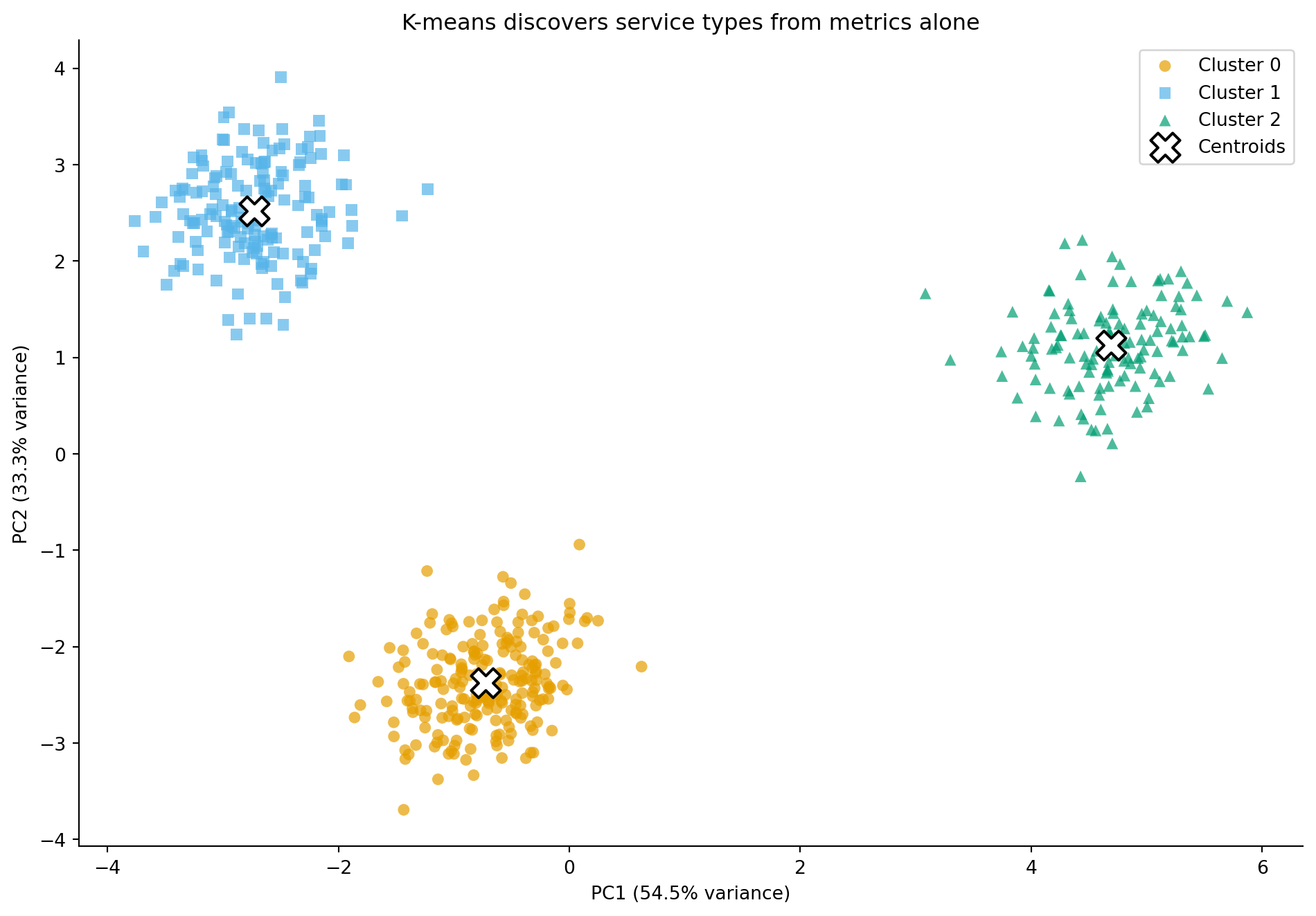
#| fig-cap: "K-means with K=3 applied to the PCA-projected telemetry data. The algorithm discovers three clusters that closely match the true service types — without any access to the labels."
#| fig-alt: "Scatter plot showing the PCA projection of 500 microservices coloured by K-means cluster assignment (K=3). Three distinct groups are visible, closely matching the web, database, and batch service types from the original simulation. Cluster centroids are marked with large white X symbols at the geometric centre of each cluster."
from sklearn.cluster import KMeans

kmeans = KMeans(n_clusters=3, random_state=42, n_init=10)
cluster_labels = kmeans.fit_predict(X_scaled)

# Colour-blind safe palette (Okabe-Ito) with distinct markers
colours = ['#0072B2', '#E69F00', '#009E73']
markers = ['o', 's', '^']

fig, ax = plt.subplots(figsize=(10, 7))
fig.patch.set_alpha(0)
ax.patch.set_alpha(0)
for k in range(3):
    mask = cluster_labels == k
    ax.scatter(X_pca[mask, 0], X_pca[mask, 1],
               c=colours[k], marker=markers[k],
               label=f'Cluster {k}', alpha=0.7, edgecolor='none', s=40)

# Project centroids onto PCA space for plotting
centroids_pca = pca.transform(kmeans.cluster_centers_)
ax.scatter(centroids_pca[:, 0], centroids_pca[:, 1],
           c='white', edgecolors='black', linewidths=1.5,
           marker='X', s=250, zorder=5, label='Centroids')

ax.set_xlabel(f'PC1 ({pca.explained_variance_ratio_[0]:.1%} variance)')
ax.set_ylabel(f'PC2 ({pca.explained_variance_ratio_[1]:.1%} variance)')
ax.set_title('K-means discovers service types from metrics alone')
ax.legend()
ax.spines[['top', 'right']].set_visible(False)
plt.tight_layout()
plt.show()
```
K-means has recovered the three service types with no access to the ground-truth labels. But how well do the discovered clusters match the actual types? Since we have labels for this simulated data, we can check, though in real unsupervised scenarios this luxury doesn't exist.
```{python}
#| label: kmeans-vs-truth
#| echo: true
# Cross-tabulate cluster assignments against true labels
ct = pd.crosstab(telemetry['service_type'], cluster_labels,
                 rownames=['True type'], colnames=['K-means cluster'])
print(ct)
```
The cross-tabulation should show strong agreement: most observations from each true type land in the same cluster. The clusters may be numbered differently (cluster 0 might correspond to "database" rather than "web"), because K-means doesn't know anything about labels. What matters is that each cluster is dominated by a single true type.
Note that K-means requires you to standardise your features first, for the same reason regularisation does (@sec-ridge): the algorithm uses Euclidean distance, and features on larger scales would dominate the distance calculation. We standardised with `StandardScaler` before fitting, so all metrics contribute equally.
::: {.callout-note}
## Engineering Bridge
K-means is a **facility location problem** — the same optimisation that arises when choosing where to place CDN edge nodes or data centre regions. Given $n$ user locations, choose $K$ facility positions to minimise the total distance between each user and their nearest facility. The assignment step is routing (each user goes to the nearest facility); the update step is repositioning (move each facility to the centre of its assigned users). Engineers who have thought about CDN PoP topology or warehouse placement will recognise this immediately. Where the analogy breaks down: facility location operates over physical geography with fixed costs; K-means operates over a feature space where "distance" is a modelling choice, not a physical fact.
:::
## Choosing K: how many clusters? {#sec-choosing-k}
K-means requires you to specify $K$ upfront. In our example, we chose $K = 3$ because we knew the data had three service types. In practice, you rarely have this luxury. Two common approaches help you choose.
The **elbow method** runs K-means for a range of $K$ values and plots WCSS against $K$. As $K$ increases, WCSS always decreases (more clusters means shorter distances to centroids), but at some point the rate of improvement diminishes sharply — the "elbow." Beyond that point, additional clusters are splitting real groups rather than capturing genuine structure.
The **silhouette score** measures how well each observation fits its assigned cluster versus the next-best alternative. For each point, the silhouette is:
$$
s(i) = \frac{b(i) - a(i)}{\max(a(i), b(i))}
$$
where $a(i)$ is the mean distance from point $i$ to other points in its cluster (cohesion), and $b(i)$ is the mean distance to points in the nearest neighbouring cluster (separation). The score ranges from $-1$ to $+1$: values near $+1$ mean the point is well matched to its cluster and poorly matched to others; values near $0$ mean it sits on the boundary between clusters; negative values indicate a likely misassignment. @sec-metrics-index lists silhouette alongside the other unsupervised and supervised evaluation metrics in this book.
```{python}
#| label: fig-elbow-silhouette
#| echo: true
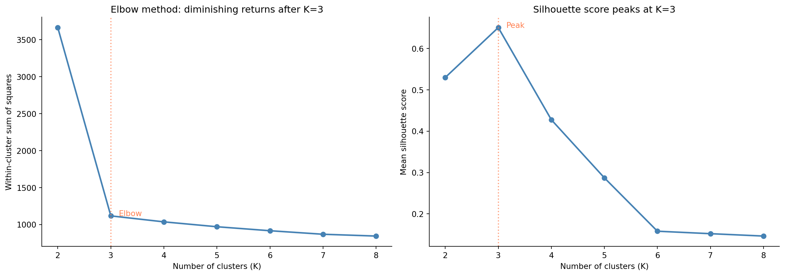
#| fig-cap: "Elbow plot (left) and silhouette score (right) for $K = 2$ to $8$. Both methods point to $K = 3$ as the best choice — WCSS shows a clear elbow, and the silhouette score peaks."
#| fig-alt: "Two-panel figure. First panel: line chart of within-cluster sum of squares (WCSS) versus K from 2 to 8, showing a steep decline from K=2 to K=3 then a much flatter decline, with a vertical dashed line at K=3 marking the elbow. Second panel: line chart of mean silhouette score versus K, peaking at K=3 with a value around 0.65, with a vertical dashed line at K=3 marking the peak. Both panels suggest K=3 as the optimal number of clusters."
from sklearn.metrics import silhouette_score

K_range = range(2, 9)
inertias = []
silhouettes = []

for k in K_range:
    km = KMeans(n_clusters=k, random_state=42, n_init=10)
    labels = km.fit_predict(X_scaled)
    inertias.append(km.inertia_)
    silhouettes.append(silhouette_score(X_scaled, labels))

k_values = list(K_range)
fig, (ax1, ax2) = plt.subplots(1, 2, figsize=(14, 5))
fig.patch.set_alpha(0)
ax1.patch.set_alpha(0)
ax2.patch.set_alpha(0)

ax1.plot(k_values, inertias, 'o-', color='#0072B2', linewidth=2)
ax1.axvline(3, color='#E69F00', linestyle=':', alpha=0.7, linewidth=1.5)
ax1.annotate('Elbow', xy=(3.15, inertias[k_values.index(3)]),
             fontsize=10, color='#E69F00')
ax1.set_xlabel('Number of clusters (K)')
ax1.set_ylabel('Within-cluster sum of squares')
ax1.set_title('Elbow method: diminishing returns after K=3')
ax1.spines[['top', 'right']].set_visible(False)

ax2.plot(k_values, silhouettes, 'o-', color='#0072B2', linewidth=2)
ax2.axvline(3, color='#E69F00', linestyle=':', alpha=0.7, linewidth=1.5)
ax2.annotate('Peak', xy=(3.15, silhouettes[k_values.index(3)]),
             fontsize=10, color='#E69F00')
ax2.set_xlabel('Number of clusters (K)')
ax2.set_ylabel('Mean silhouette score')
ax2.set_title('Silhouette score peaks at K=3')
ax2.spines[['top', 'right']].set_visible(False)

plt.tight_layout()
plt.show()
```
Both diagnostics converge on $K = 3$ for this dataset. In practice, these heuristics don't always give such a clear signal: the elbow can be gradual rather than sharp, and silhouette scores may vary little across several values of $K$. When the data's true structure doesn't consist of neatly separated spherical clusters, these methods may disagree or provide ambiguous guidance. Clustering is inherently more subjective than supervised learning: there is no ground-truth $y$ to validate against. The silhouette thresholds sometimes cited (above 0.5 is "good," below 0.25 is "poor") are rough guides, not standards; interpret them relative to your data's complexity.
::: {.callout-tip}
## Author's Note
The subjectivity of clustering bothered me more than anything else in this part of the book. In supervised learning, you have a test set and a clear metric: your model either predicts well or it doesn't. In clustering, "good" is partly a matter of opinion. Two analysts could legitimately argue for different values of $K$, and neither would be wrong in any provable sense. The most useful reframe is to think of clustering as *exploratory* rather than *confirmatory*: it generates hypotheses about structure in your data, not conclusions. The value of clustering is in the patterns it reveals and the questions it raises, not in a definitive answer.
:::
## K-means assumptions and limitations {#sec-kmeans-limitations}
K-means makes implicit assumptions that matter in practice. It assumes clusters are roughly **spherical** (equidistant in all directions from the centroid) and roughly **equal in density** (similar spread around each centroid). When these assumptions hold, K-means performs well. When they don't — elongated clusters, clusters of very different densities, or clusters with irregular shapes — the algorithm can produce misleading results.
K-means is also sensitive to **initialisation**. The k-means++ initialisation strategy (the default in scikit-learn) mitigates this significantly, and running the algorithm multiple times with different initialisations (`n_init=10` is the default) helps ensure you don't get stuck in a poor local minimum. K-means is an alternating optimisation algorithm: each step reduces WCSS, but the final result depends on where you started. Gaussian mixture models (GMMs), which we don't cover here, extend K-means with probabilistic (soft) assignments: each observation gets a probability of belonging to each cluster, which naturally handles ambiguous boundary points.
Finally, K-means assigns *every* observation to a cluster. There's no concept of "this point doesn't belong to any group": outliers and noise points get absorbed into the nearest cluster, potentially distorting centroids and cluster boundaries. For data with genuine outliers, this is a real problem.
## Hierarchical clustering: the dendrogram {#sec-hierarchical}
**Hierarchical clustering** takes a fundamentally different approach. Instead of partitioning the data into a fixed number of groups, it builds a tree of nested clusters — a **dendrogram** — that shows how observations merge together at different levels of similarity.
The most common variant, **agglomerative** (bottom-up) clustering, starts with each observation as its own cluster (500 clusters for 500 observations), finds the two closest clusters and merges them, and repeats until all observations belong to a single cluster. The result is a hierarchy: at the bottom, every point is its own cluster; at the top, everything is one cluster; and every level in between represents a different granularity of grouping. You choose the number of clusters by "cutting" the dendrogram at a particular height.
The key decision is how to measure the distance between two *clusters* (not just two points); this is called the **linkage** criterion. **Ward's method** minimises the increase in the total within-cluster sum of squares (the same WCSS quantity K-means minimises) when two clusters merge, tending to produce compact, spherical clusters; it's often the default choice. **Complete linkage** uses the maximum distance between any pair of points in the two clusters, producing clusters of similar diameter. **Average linkage** uses the mean distance between all pairs of points across the two clusters. **Single linkage** uses the minimum distance, which can detect elongated clusters but is prone to "chaining", absorbing outliers and creating thin, straggling clusters.
```{python}
#| label: fig-dendrogram
#| echo: true
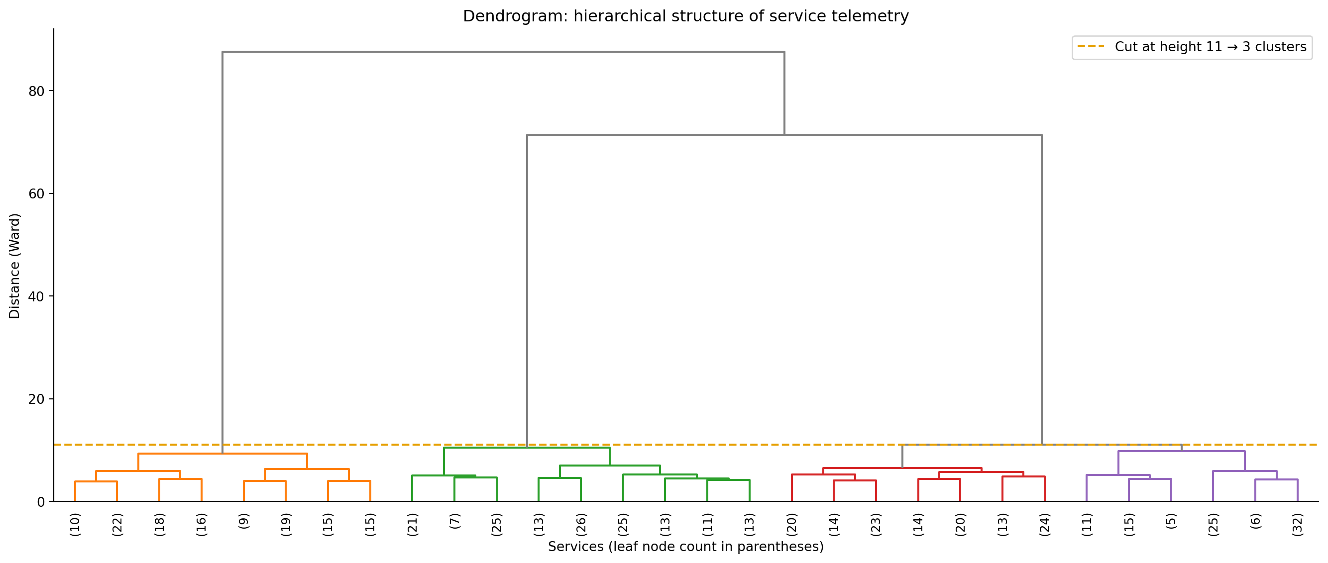
#| fig-cap: "Dendrogram of the telemetry data using Ward's linkage (truncated to 30 leaf nodes for readability). The three major branches correspond to the three service types. The dashed line shows where cutting the tree yields three clusters."
#| fig-alt: "Dendrogram showing hierarchical clustering of 500 services using Ward's linkage. The tree has three major branches that merge at heights above the cut line. A horizontal dashed line marks where cutting produces three clusters. Branches below the cut are coloured; branches above are grey."
from scipy.cluster.hierarchy import dendrogram, linkage, fcluster

Z = linkage(X_scaled, method='ward')

# Compute cut height dynamically: the merge distance that yields 3 clusters
cut_height = Z[-3, 2]

fig, ax = plt.subplots(figsize=(14, 6))
fig.patch.set_alpha(0)
ax.patch.set_alpha(0)
dendrogram(Z, truncate_mode='lastp', p=30, leaf_rotation=90,
           leaf_font_size=9, ax=ax, color_threshold=cut_height,
           above_threshold_color='grey')
ax.axhline(y=cut_height, color='#E69F00', linestyle='--', linewidth=1.5,
           label=f'Cut at height {cut_height:.0f} → 3 clusters')
ax.set_xlabel('Services (leaf node count in parentheses)')
ax.set_ylabel('Distance (Ward)')
ax.set_title('Dendrogram: hierarchical structure of service telemetry')
ax.legend()
ax.spines[['top', 'right']].set_visible(False)
plt.tight_layout()
plt.show()
```
The dendrogram reveals more than just "there are three clusters." It shows the *hierarchy* of similarity: which groups are most alike and which are most distinct. If the three-cluster cut produces groups that are too coarse, you could cut lower to get finer sub-groups, perhaps distinguishing read-heavy databases from write-heavy ones, or CPU-bound batch jobs from I/O-bound batch jobs.
```{python}
#| label: fig-hierarchical-scatter
#| echo: true
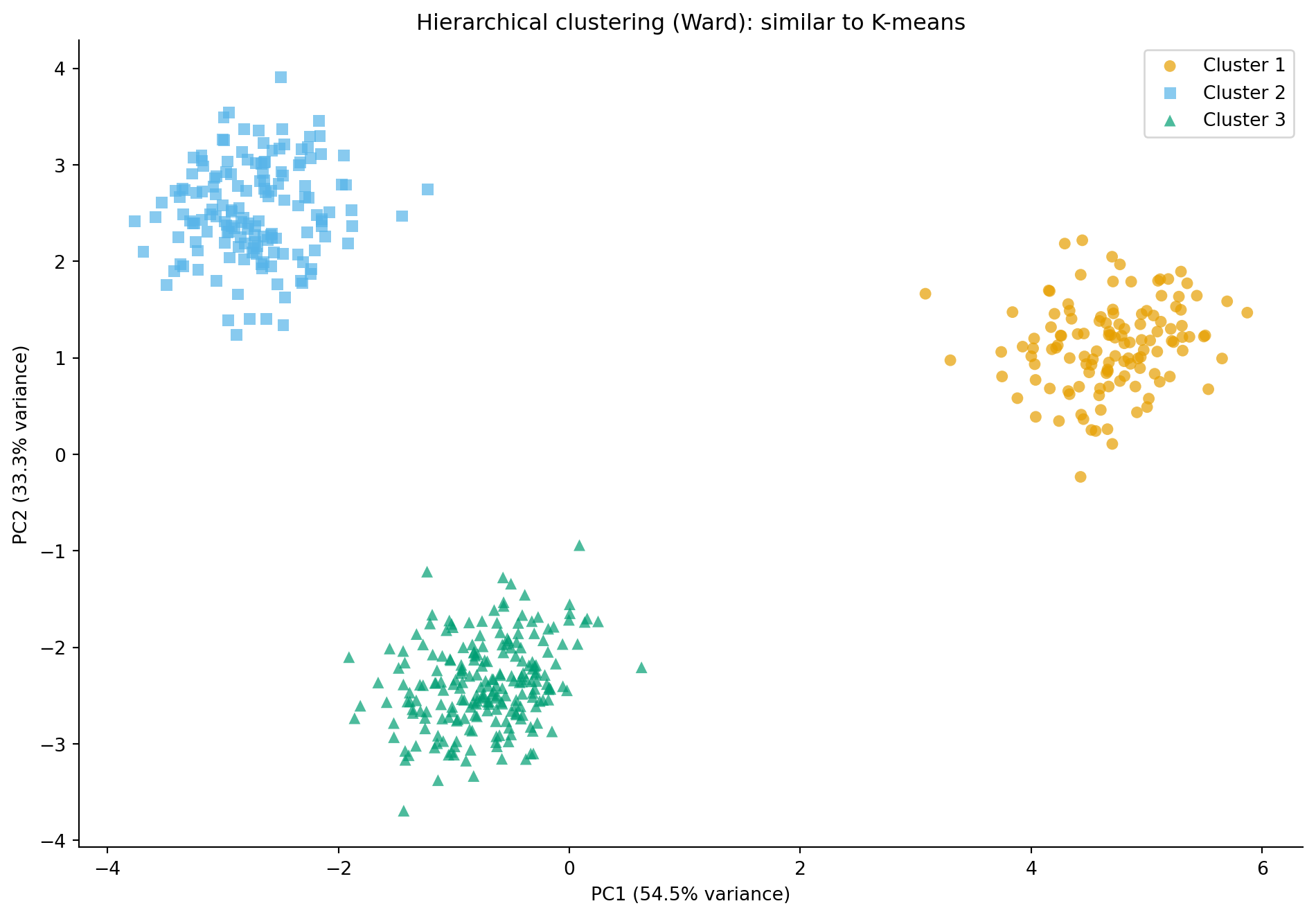
#| fig-cap: "Hierarchical clustering (Ward's linkage, 3 clusters) agrees closely with K-means, confirming the structure is genuine rather than an artefact of the method. Unlike K-means, hierarchical clustering has no centroids to plot."
#| fig-alt: "Scatter plot of the PCA projection for 500 microservices, with points coloured and shaped by hierarchical cluster assignment (Ward's linkage, 3 clusters). Three groups are spatially separated: circles in one region, squares in another, and triangles in a third. The arrangement is nearly identical to the K-means result."
hier_labels = fcluster(Z, t=3, criterion='maxclust')

fig, ax = plt.subplots(figsize=(10, 7))
fig.patch.set_alpha(0)
ax.patch.set_alpha(0)
for k in range(1, 4):
    mask = hier_labels == k
    ax.scatter(X_pca[mask, 0], X_pca[mask, 1],
               c=colours[k - 1], marker=markers[k - 1],
               label=f'Cluster {k}', alpha=0.7, edgecolor='none', s=40)

ax.set_xlabel(f'PC1 ({pca.explained_variance_ratio_[0]:.1%} variance)')
ax.set_ylabel(f'PC2 ({pca.explained_variance_ratio_[1]:.1%} variance)')
ax.set_title('Hierarchical clustering (Ward): similar to K-means')
ax.legend()
ax.spines[['top', 'right']].set_visible(False)
plt.tight_layout()
plt.show()
```
Both algorithms agree on this dataset — confirming the clusters are genuine rather than artefacts of the method — but their computational costs differ dramatically. With $n$ observations, Ward's linkage in `scipy` runs in $O(n^2)$ time and memory, which makes it impractical for more than a few thousand observations. For 10,000 services, the distance matrix alone consumes roughly 400 MB; by 100,000 services it requires around 40 GB. K-means, by contrast, scales as $O(nK)$ per iteration and handles large datasets comfortably. For truly large-scale clustering, scikit-learn's `MiniBatchKMeans` processes data in batches without loading the full distance matrix.
## DBSCAN: density-based clustering {#sec-dbscan}
Both K-means and hierarchical clustering assume that clusters are roughly spherical; they work best when groups form compact, convex shapes in feature space. **DBSCAN** (Density-Based Spatial Clustering of Applications with Noise) drops this assumption entirely. It defines clusters as *dense regions* separated by *sparse regions*, which lets it discover clusters of arbitrary shape.
DBSCAN has two parameters: **`eps`** ($\varepsilon$), the radius of the neighbourhood around each point, and **`min_samples`**, the minimum number of points within `eps` distance to qualify a point as a **core point**, the backbone of a cluster. (This $\varepsilon$ is unrelated to the error term $\varepsilon$ from @sec-determinism; it's the conventional symbol for the DBSCAN radius parameter, matching scikit-learn's `eps` argument.)
The algorithm classifies every point into one of three categories. **Core points** have at least `min_samples` neighbours within distance `eps` and form the dense centres of clusters. **Border points** fall within `eps` of a core point but don't have enough neighbours to be core points themselves; they're assigned to the nearest core point's cluster. **Noise points** don't fall within `eps` of any core point and are left unassigned, labelled as $-1$.
This last property is DBSCAN's most distinctive feature: it can identify observations that don't belong to *any* cluster. K-means forces every point into a group; DBSCAN allows outliers to be outliers.
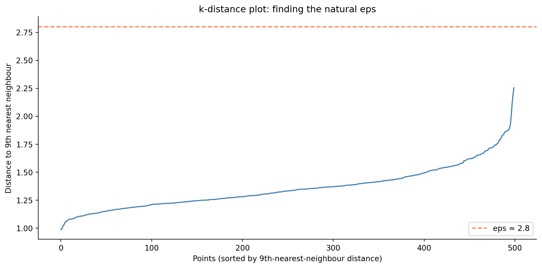
The trade-off is that DBSCAN's two parameters can be difficult to tune. Too small an `eps` and everything is noise; too large and distinct clusters merge. A common heuristic is to plot the sorted distances to the $k$-th nearest neighbour (setting $k = \texttt{min\_samples}$) and look for an elbow, using that distance as `eps`.
```{python}
#| label: fig-dbscan-eps-selection
#| echo: true
#| fig-cap: "The k-distance plot helps choose DBSCAN's eps parameter. The distance to each point's 10th nearest neighbour is sorted in ascending order; the curve rises gently for most points then turns upward near its tail, reaching just over 2.2 at the far right. The knee is around 1.5, and we pick an eps just above it — here `eps ≈ 1.5` — as a natural radius."
#| fig-alt: "Line chart showing sorted 10th-nearest-neighbour distances for 500 services. The curve rises slowly for most points then turns upward steeply for the last few dozen, reaching just over 2.2 at the far right. A horizontal dashed line at approximately 1.5 sits just above the knee, marking the eps chosen for DBSCAN."
from sklearn.neighbors import NearestNeighbors

# k = min_samples = 10
nn = NearestNeighbors(n_neighbors=10)
nn.fit(X_scaled)
distances, _ = nn.kneighbors(X_scaled)
k_distances = np.sort(distances[:, -1])

fig, ax = plt.subplots(figsize=(10, 5))
fig.patch.set_alpha(0)
ax.patch.set_alpha(0)
ax.plot(k_distances, color='#0072B2', linewidth=1.5)
ax.axhline(1.5, color='#E69F00', linestyle='--', linewidth=1.5,
           label='eps ≈ 1.5')
ax.set_xlabel('Points (sorted by 10th-nearest-neighbour distance)')
ax.set_ylabel('Distance to 10th nearest neighbour')
ax.set_title('k-distance plot: finding the natural eps')
ax.legend()
ax.spines[['top', 'right']].set_visible(False)
plt.tight_layout()
plt.show()
```
```{python}
#| label: fig-dbscan
#| echo: true
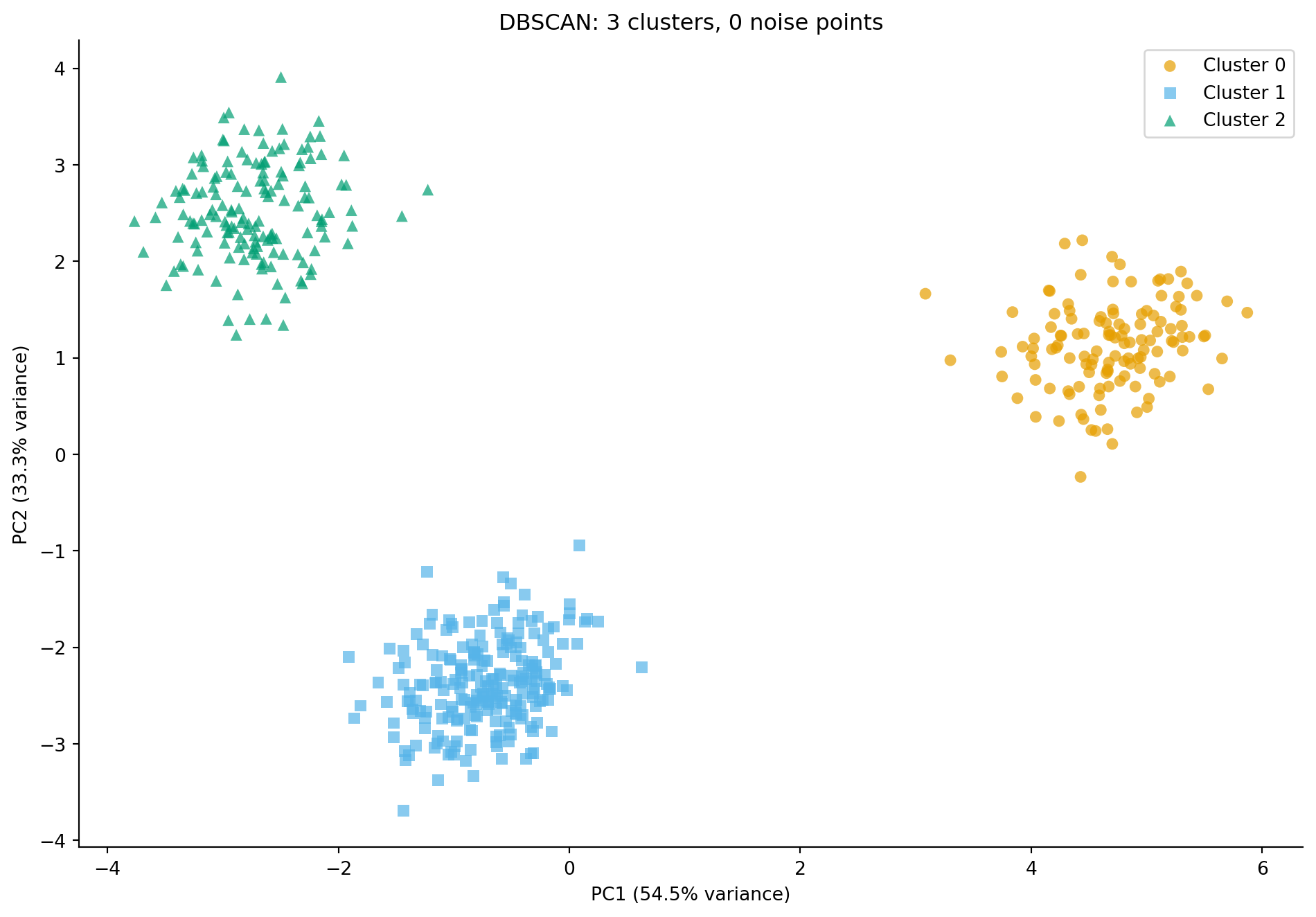
#| fig-cap: "DBSCAN applied to the telemetry data. It discovers clusters automatically (coloured) and identifies noise points (grey crosses) that sit between the main groups — observations the algorithm could not confidently assign to any cluster."
#| fig-alt: "Scatter plot of the PCA projection with points coloured by DBSCAN cluster assignment. Three main clusters are visible in distinct colours with distinct marker shapes, closely matching the true service types. A small number of grey cross-shaped points scattered between clusters represent noise points that DBSCAN did not assign to any cluster."
from sklearn.cluster import DBSCAN

dbscan = DBSCAN(eps=1.5, min_samples=10)
db_labels = dbscan.fit_predict(X_scaled)

n_clusters = len(set(db_labels) - {-1})
n_noise = (db_labels == -1).sum()
print(f"DBSCAN found {n_clusters} clusters and {n_noise} noise points")

fig, ax = plt.subplots(figsize=(10, 7))
fig.patch.set_alpha(0)
ax.patch.set_alpha(0)

# Plot noise points first (grey crosses)
noise_mask = db_labels == -1
if noise_mask.any():
    ax.scatter(X_pca[noise_mask, 0], X_pca[noise_mask, 1],
               c='grey', marker='x', alpha=0.8, s=60,
               linewidths=1.5, label='Noise')

# Plot clusters
for k in range(n_clusters):
    mask = db_labels == k
    ax.scatter(X_pca[mask, 0], X_pca[mask, 1],
               c=colours[k % len(colours)], marker=markers[k % len(markers)],
               label=f'Cluster {k}', alpha=0.7, edgecolor='none', s=40)

ax.set_xlabel(f'PC1 ({pca.explained_variance_ratio_[0]:.1%} variance)')
ax.set_ylabel(f'PC2 ({pca.explained_variance_ratio_[1]:.1%} variance)')
ax.set_title(f'DBSCAN: {n_clusters} clusters, {n_noise} noise points')
ax.legend()
ax.spines[['top', 'right']].set_visible(False)
plt.tight_layout()
plt.show()
```
DBSCAN's ability to flag noise points is valuable when your data contains outliers: services that don't fit any typical profile, customer accounts with anomalous usage, or incidents that defy categorisation. In an engineering context, these outliers are often the most interesting observations: the service that behaves like neither a web server nor a database might be the one that needs attention.
::: {.callout-note}
## Engineering Bridge
DBSCAN's core/border/noise classification parallels how **monitoring systems triage hosts**. Many SRE platforms distinguish between normal hosts (healthy, exhibiting expected behaviour), marginal hosts (within the cluster but underperforming), and orphan hosts (completely outside expected patterns, flagged for investigation). The `min_samples` parameter maps to a **quorum** concept from distributed consensus — a node needs enough peers exhibiting similar behaviour to be considered part of a healthy group. Isolated nodes with no quorum are suspected faulty. Where the analogy breaks down: DBSCAN classifies by spatial density in a static feature space, while monitoring triage operates over time-varying metrics with causal context that DBSCAN cannot capture.
:::
## Comparing algorithms side by side {#sec-clustering-comparison}
Each clustering algorithm makes different assumptions and has different strengths. Let's see all three approaches together.
```{python}
#| label: fig-clustering-comparison
#| echo: true
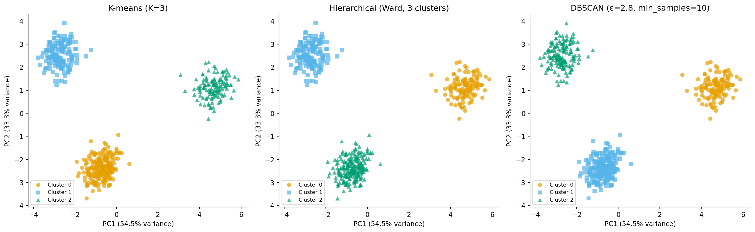
#| fig-cap: "Three clustering approaches on the same data. K-means and hierarchical clustering produce similar partitions; DBSCAN additionally identifies noise points between clusters. Cluster colours are assigned by integer index and do not correspond across panels — the same colour in different panels may represent different service types."
#| fig-alt: "Three-panel scatter plot comparing K-means (first panel), hierarchical Ward (second panel), and DBSCAN (third panel) clustering on the PCA projection. The first and second panels show three well-separated clusters with distinct marker shapes. The third panel shows the same three clusters plus a small number of grey cross-shaped noise points between them. Each panel has labelled PC1 and PC2 axes with variance percentages."
fig, axes = plt.subplots(1, 3, figsize=(16, 5))
fig.patch.set_alpha(0)
for ax in axes:
    ax.patch.set_alpha(0)

all_labels = [
    (cluster_labels, 'K-means (K=3)'),
    (hier_labels - 1, 'Hierarchical (Ward, 3 clusters)'),
    (db_labels, 'DBSCAN (ε=1.5, min_samples=10)'),
]

for ax, (labels, title) in zip(axes, all_labels):
    unique = sorted(set(labels))
    for k in unique:
        mask = labels == k
        if k == -1:
            ax.scatter(X_pca[mask, 0], X_pca[mask, 1],
                       c='grey', marker='x', alpha=0.8, s=60,
                       linewidths=1.5, label='Noise')
        else:
            ax.scatter(X_pca[mask, 0], X_pca[mask, 1],
                       c=colours[k % len(colours)],
                       marker=markers[k % len(markers)],
                       label=f'Cluster {k}', alpha=0.7,
                       edgecolor='none', s=40)
    ax.set_xlabel(f'PC1 ({pca.explained_variance_ratio_[0]:.1%} variance)')
    ax.set_ylabel(f'PC2 ({pca.explained_variance_ratio_[1]:.1%} variance)')
    ax.set_title(title)
    ax.legend(fontsize=8, loc='lower left')
    ax.spines[['top', 'right']].set_visible(False)

plt.tight_layout()
plt.show()
```
For well-separated, roughly spherical clusters like our telemetry data, all three algorithms give sensible results. The differences become more pronounced with messier real-world data:
: Comparison of three clustering algorithms by key properties {#tbl-clustering-comparison}
| Property | K-means | Hierarchical (Ward) | DBSCAN |
| -------: | :------ | :------------------ | :----- |
| Cluster shape assumption | Spherical | Depends on linkage | Arbitrary |
| Must specify $K$ | Yes | Cut height or $K$ | No (discovers $K$) |
| Handles noise/outliers | No (assigns all) | No (assigns all) | Yes (labels noise) |
| Scalability | $O(nK)$ per iteration — fast | $O(n^2)$ time and memory — slow | $O(n \log n)$ with spatial index; $O(n^2)$ in high dimensions |
| Deterministic | No (random init) | Yes | Yes |
## Evaluating clusters without labels {#sec-cluster-evaluation}
In supervised learning, evaluation is straightforward: compare predictions to known labels. In clustering, we usually don't have labels — that's the whole point. Several **internal** metrics evaluate cluster quality using only the data itself.
The **silhouette score** (introduced in @sec-choosing-k) works for any clustering algorithm, not just K-means. It measures how well-separated clusters are on average.
When you *do* have ground-truth labels (as we do with this simulated data), **external** metrics compare discovered clusters to the true groups. The **adjusted Rand index** (ARI) measures agreement between two partitions, adjusted for chance. An ARI of 1.0 means perfect agreement; 0.0 means no better than random. ARI is summarised, with its label requirement and trap cases, in @sec-metrics-index.
```{python}
#| label: cluster-evaluation
#| echo: true
from sklearn.metrics import silhouette_score, adjusted_rand_score

# Internal evaluation (no labels needed)
# Silhouette for DBSCAN excludes noise — noise points have no cluster assignment
db_mask = db_labels != -1
print('Silhouette scores (internal):')
print(f"  K-means:      {silhouette_score(X_scaled, cluster_labels):.3f}")
print(f"  Hierarchical: {silhouette_score(X_scaled, hier_labels):.3f}")
if db_mask.sum() > 0 and len(set(db_labels[db_mask])) > 1:
    print(f"  DBSCAN:       {silhouette_score(X_scaled[db_mask], db_labels[db_mask]):.3f}"
          '  (noise points excluded)')

# External evaluation (ground truth available)
# ARI computed on ALL observations for fair comparison —
# DBSCAN noise points (label -1) form their own "cluster"
true_numeric = type_labels.codes
print('\nAdjusted Rand Index (vs true labels):')
print(f"  K-means:      {adjusted_rand_score(true_numeric, cluster_labels):.3f}")
print(f"  Hierarchical: {adjusted_rand_score(true_numeric, hier_labels):.3f}")
print(f"  DBSCAN:       {adjusted_rand_score(true_numeric, db_labels):.3f}")
```
High silhouette scores and ARI values confirm that all three algorithms have successfully recovered the latent structure. The DBSCAN ARI is computed over all observations (including noise points, which are treated as their own group), making it directly comparable to the other two algorithms. In real applications where you don't have ground-truth labels, silhouette scores and visual inspection of the clusters (projected via PCA or t-SNE from @sec-tsne) are your primary tools for assessing quality.
::: {.callout-tip}
## Author's Note
The evaluation problem in clustering was a genuine blind spot for me. Coming from supervised learning, I kept wanting a "test set accuracy" equivalent. There isn't one. The silhouette score and ARI are useful, but they measure different things — internal cohesion vs. agreement with external labels — and neither tells you whether the clusters are *meaningful*. You can find perfectly well-separated clusters that correspond to nothing useful, and messy, overlapping clusters that reveal a genuinely important business distinction. The numbers guide you; domain knowledge decides.
:::
## Clustering in practice {#sec-clustering-practical}
Before applying clustering to real data, there are several considerations worth checking, the same way you'd review a checklist before deploying a new service.
All three algorithms in this chapter use distance metrics, so **feature scaling** is essential. Unscaled features with larger ranges will dominate the distance calculations. Always standardise before clustering, just as with regularised models (@sec-ridge) and PCA (@sec-variance-as-information).
In very high-dimensional spaces, the "curse of dimensionality" makes distances less meaningful: all points become roughly equidistant. If you have hundreds of features, consider applying PCA first to reduce dimensionality before clustering. The combination of PCA followed by K-means is a common and effective pipeline. Note that DBSCAN's $O(n \log n)$ scalability (from its spatial index) degrades toward $O(n^2)$ in high dimensions where the index becomes ineffective.
For K-means specifically, check whether cluster assignments are **stable** across runs. Run with different random seeds (scikit-learn's `n_init` parameter handles this) and compare the results using ARI between runs: a high ARI (close to 1.0) means the structure is robust, not just a matter of which initialisation happened to win. If different initialisations produce very different clusters, the structure may be weak.
Finally, the clusters are only useful if you can **interpret** them in domain terms. The cluster profile (computed in the following code block), showing mean values for the most discriminating features, is usually the first thing to share with domain experts. Engineers who routinely compute per-group metric means in A/B analysis will recognise this pattern: compute per-cluster means, look for the largest differences, and name the groups.
```{python}
#| label: cluster-profiles
#| echo: true
# Compute mean profiles for each K-means cluster
telemetry['cluster'] = cluster_labels
cluster_means = telemetry.groupby('cluster')[feature_names].mean().T
cluster_means.columns = [f'Cluster {k}' for k in cluster_means.columns]

# Show the features with the largest differences across clusters
profile_range = cluster_means.max(axis=1) - cluster_means.min(axis=1)
top_features = profile_range.nlargest(6).index

print('Cluster profiles (top 6 distinguishing features):')
print(cluster_means.loc[top_features].round(1).to_string())
```
One cluster likely has high latency, high CPU, and high thread utilisation: the batch processors. Another has high memory and disk usage: the databases. The third has high network throughput: the web servers. These interpretations come from domain knowledge, not the algorithm. And if you have labels available, you should use them; clustering is for when you don't. A common mistake is reaching for unsupervised clustering when a supervised classification model would be more appropriate and more reliable.
## Summary {#sec-clustering-summary}
1. **Clustering is inherently exploratory.** It discovers groups in data without a target variable and generates hypotheses about structure, not definitive answers. Domain knowledge determines whether clusters are meaningful — metrics alone cannot.
2. **K-means partitions data into $K$ spherical clusters** by minimising within-cluster distance. It is fast and effective but requires specifying $K$ upfront and assumes compact clusters of similar density.
3. **Hierarchical clustering builds a tree of nested clusters** (a dendrogram) that reveals structure at multiple resolutions. It is more informative than K-means but computationally expensive for large datasets ($O(n^2)$ for Ward's linkage).
4. **DBSCAN finds clusters of arbitrary shape** by identifying dense regions, and uniquely among the three algorithms, it can flag observations as noise. It requires tuning `eps` and `min_samples` rather than specifying $K$.
5. **Evaluating clusters is inherently subjective.** Internal metrics (silhouette score) and external metrics (adjusted Rand index) provide quantitative guidance, but two analysts may legitimately disagree on the best partition.
In the next chapter, *Time series: modelling sequential data*, we shift from static snapshots to data that evolves over time: sequences where the order of observations matters as much as their values.
## Exercises {#sec-clustering-exercises}
1. Run K-means on the telemetry data with $K = 2, 4, 5, 6$. For each, compute the silhouette score and visualise the clusters on the PCA projection. At $K = 5$ or $K = 6$, which true service types get split into sub-clusters?
2. Apply DBSCAN to the telemetry data with `min_samples=10` and `eps` values of 1.5, 2.8, and 5.0. How does `eps` affect the number of clusters found and the number of noise points? Plot the results side by side.
3. Build a clustering pipeline that first reduces the telemetry data to 3 PCA components, then applies K-means with $K = 3$. Compare the ARI of this pipeline against K-means applied to the full 15-dimensional standardised data. Does dimensionality reduction help or hurt clustering quality?
4. **Conceptual:** Your team clusters customer support tickets by text similarity and discovers five groups. A colleague argues that the "right" number of clusters is seven, based on the silhouette score. Another says three, because it aligns with the company's existing product categories. Who is right? How would you resolve this disagreement?
5. **Conceptual:** You extend the telemetry clustering to include services that were recently spun up for a canary deployment and don't yet have a stable resource profile. Why would K-means assignment of these services produce misleading cluster centroids? How would you detect this, and what would DBSCAN's output reveal instead?