---
# Content: CC BY-NC-SA 4.0 | Code: MIT - see /LICENSE.md
title: "Tree-based models: when straight lines aren't enough"
---
{{< include /_common-imports.qmd >}}
## The limits of linearity {#sec-when-lines-fail}
Consider a production incident response team. When a server goes down, several factors influence how long it takes to resolve: CPU and memory pressure, error rates, request volume, how many services are affected, and who's on call.
Some of these relationships are non-linear in ways that matter. When CPU *and* memory are both above 70%, resolution time spikes because the interaction between the two is what kills you, not either metric alone. High request volume causes problems only beyond a threshold. A linear model can't capture these patterns without extensive manual feature engineering. Tree-based models discover them automatically.
In @sec-regression-pitfalls we saw that when the true relationship curves, a straight line systematically under-predicts in some regions and over-predicts in others. The residual plots from @sec-residual-analysis reveal the problem. This chapter introduces models that handle non-linearity naturally, without requiring you to guess the right transformation or polynomial degree up front.
```{python}
#| label: incident-data-generation
#| echo: true
#| code-fold: true
#| code-summary: "Expand to see incident data simulation (600 rows, 8 features)"
from sklearn.model_selection import train_test_split
from sklearn.linear_model import LinearRegression
from sklearn.metrics import root_mean_squared_error

rng = np.random.default_rng(42)
n = 600

incident_data = pd.DataFrame({
    'cpu_pct': rng.uniform(20, 99, n),
    'memory_pct': rng.uniform(20, 99, n),
    'error_rate': rng.exponential(2, n).clip(0, 30),
    'request_volume_k': rng.uniform(1, 100, n),
    'services_affected': rng.integers(1, 12, n),
    'is_deploy_related': rng.binomial(1, 0.3, n),
    'hour_of_day': rng.integers(0, 24, n),
    'on_call_experience_yrs': rng.uniform(0.5, 15, n),
})

# Non-linear data-generating process
resolution_time = (
    30
    + 0.5 * incident_data['error_rate']
    + 3.0 * incident_data['services_affected']
    + 10 * incident_data['is_deploy_related']
    - 1.5 * incident_data['on_call_experience_yrs']
    # Non-linear interaction: both CPU and memory high causes a spike
    + 40 * ((incident_data['cpu_pct'] > 70) & (incident_data['memory_pct'] > 70)).astype(float)
    # Threshold effect: request volume only matters above 60k
    + 0.8 * np.maximum(incident_data['request_volume_k'] - 60, 0)
    # Night-time incidents take longer (reduced staffing)
    + 8 * ((incident_data['hour_of_day'] < 6) | (incident_data['hour_of_day'] > 22)).astype(float)
    + rng.normal(0, 8, n)
)
incident_data['resolution_min'] = resolution_time.clip(5)

feature_names = ['cpu_pct', 'memory_pct', 'error_rate', 'request_volume_k',
                 'services_affected', 'is_deploy_related', 'hour_of_day',
                 'on_call_experience_yrs']

X = incident_data[feature_names]
y = incident_data['resolution_min']

X_train, X_test, y_train, y_test = train_test_split(
    X, y, test_size=0.2, random_state=42
)
```
```{python}
#| label: fig-linear-baseline
#| echo: true
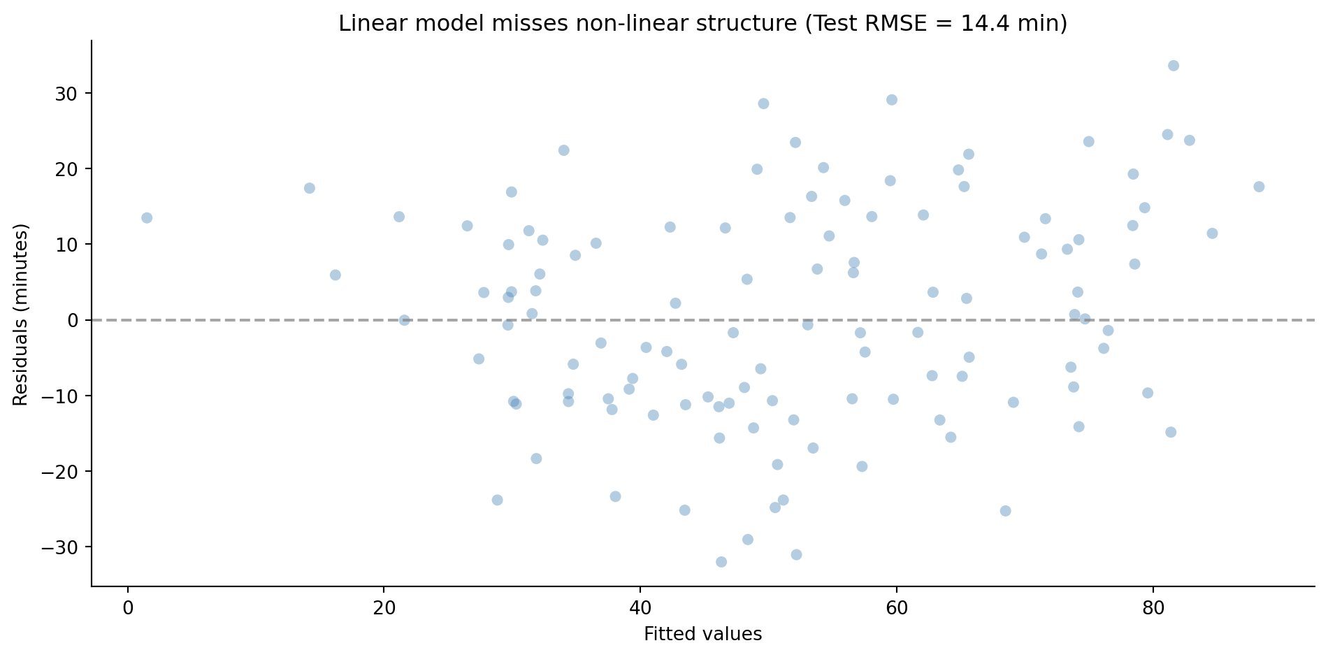
#| fig-cap: "Residuals from a linear regression on incident resolution time. The curved pattern reveals the model is missing non-linear structure in the data."
#| fig-alt: "Scatter plot of residuals versus fitted values from a linear regression model. The points show a clear curved pattern rather than random scatter, with systematic over-prediction at low fitted values and under-prediction at intermediate values, indicating model misspecification."
lr = LinearRegression().fit(X_train, y_train)
lr_train_rmse = root_mean_squared_error(y_train, lr.predict(X_train))
lr_test_rmse = root_mean_squared_error(y_test, lr.predict(X_test))

fig, ax = plt.subplots(figsize=(10, 5))
fig.patch.set_alpha(0)
ax.patch.set_alpha(0)
residuals = y_test - lr.predict(X_test)
ax.scatter(lr.predict(X_test), residuals, alpha=0.4, color='#0072B2',
           edgecolor='none')
ax.axhline(0, color='grey', linestyle='--', alpha=0.7)
ax.set_xlabel('Fitted values')
ax.set_ylabel('Residuals (minutes)')
ax.set_title(f'Linear model misses non-linear structure '
             f'(Test RMSE = {lr_test_rmse:.1f} min)')
ax.spines[['top', 'right']].set_visible(False)
plt.tight_layout()
plt.show()
```
The residual plot tells the same story we saw in @sec-residual-analysis: systematic patterns mean the model is missing structure. The linear model can't represent the CPU-memory interaction or the request volume threshold. We need something more flexible — but not so flexible that it memorises the noise, the overfitting problem from @sec-overfitting.
## Decision trees: recursive partitioning {#sec-decision-trees}
A decision tree learns a set of if-else rules from data. At each step, it picks the feature and threshold that best splits the observations into groups with more homogeneous outcomes. Then it repeats the process within each group, recursively partitioning the data into smaller and smaller regions.
If you've ever written a dispatch function, routing requests based on a chain of conditions, you've built something structurally similar. The difference is that you wrote the rules by hand based on domain knowledge, while the tree learns them from data.
For regression, "best split" means the split that most reduces the variance of the target variable within each resulting group. The tree evaluates every feature at every possible threshold, picks the one that minimises the weighted sum of child node variances (weighted by the fraction of samples in each child), and repeats. The prediction for any region is simply the mean of the training observations that fell into it. For classification, the splitting criterion changes; we'll cover that in @sec-tree-classification.
```{python}
#| label: fig-decision-tree
#| echo: true
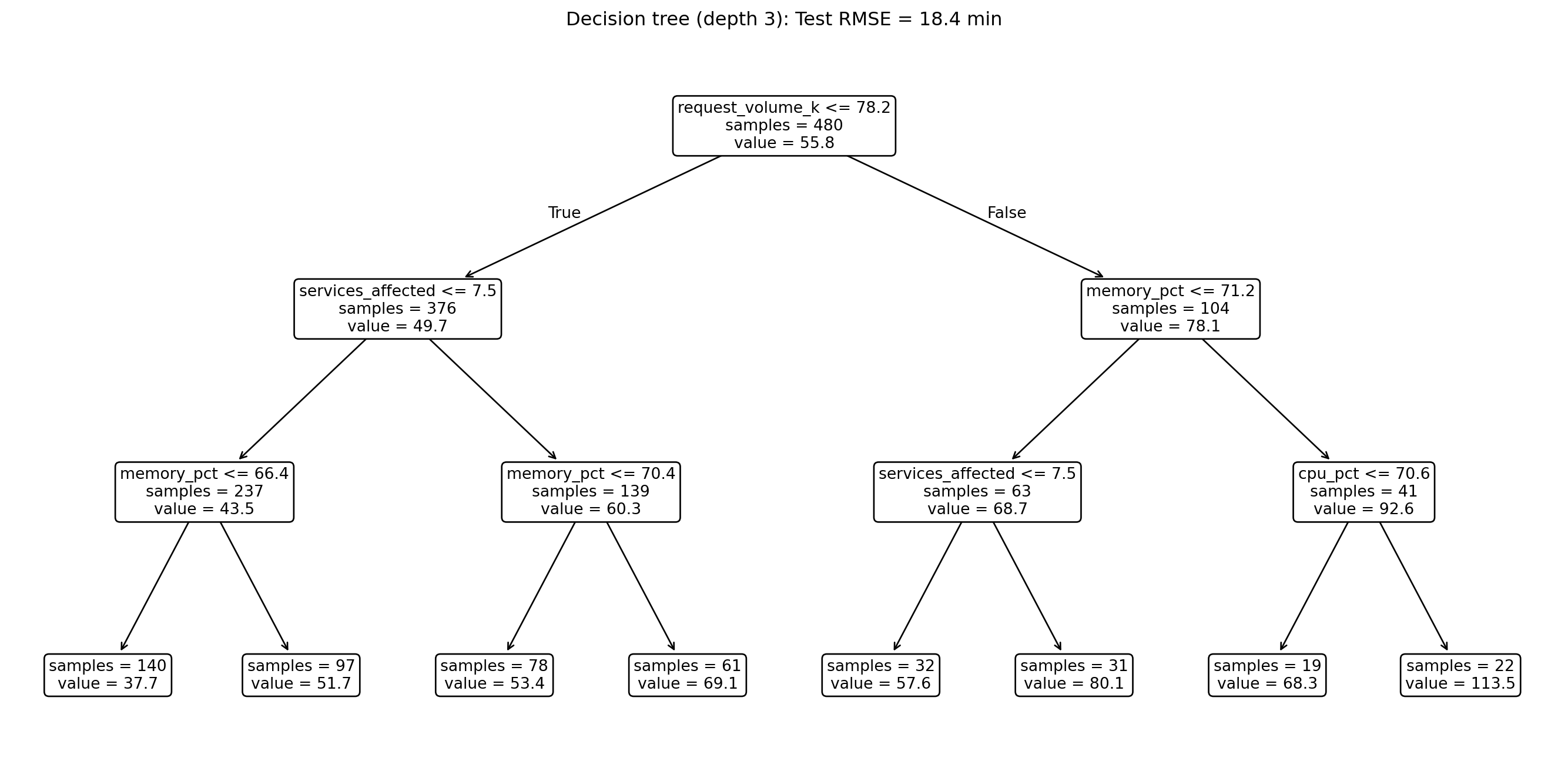
#| fig-cap: "A shallow decision tree (depth 3) for predicting incident resolution time. Each node shows the splitting rule, predicted value, and sample count."
#| fig-alt: "Tree diagram of a decision tree with depth 3. The root node splits on a feature threshold, branching into further threshold tests. Each node displays the feature threshold, predicted resolution time in minutes, and the number of training samples."
from sklearn.tree import DecisionTreeRegressor, plot_tree

dt_shallow = DecisionTreeRegressor(max_depth=3, random_state=42)
dt_shallow.fit(X_train, y_train)

dt_test_rmse = root_mean_squared_error(y_test, dt_shallow.predict(X_test))

fig, ax = plt.subplots(figsize=(14, 7))
fig.patch.set_alpha(0)
ax.patch.set_alpha(0)
plot_tree(dt_shallow, feature_names=feature_names, filled=False, rounded=True,
          fontsize=10, ax=ax, impurity=False, precision=1)
ax.set_title(f'Decision tree (depth 3): Test RMSE = {dt_test_rmse:.1f} min')
plt.tight_layout()
plt.show()
```
Even at depth 3, the tree has discovered meaningful structure: look at which features it splits on first. However, notice that the depth-3 tree's test RMSE is actually *worse* than the linear model's. With only three levels of splits, the tree has identified the non-linear patterns but hasn't had enough depth to exploit them fully. The payoff comes when we combine many such trees into an ensemble, as we'll see shortly.
::: {.callout-note}
## Engineering Bridge
A decision tree is a learned if-else chain. Instead of manually writing `if cpu > 70 and memory > 70: escalate()`, the tree discovers these conditions from data. The internal nodes are your conditionals, the branches are the execution paths, and the leaf nodes are the return values. The difference from hand-coded dispatch logic is that the tree optimises the split points to minimise prediction error across the entire training set: it's an exhaustive search over all possible if-else structures up to a given depth, something impractical to do by hand with eight features.
:::
## Overfitting in trees: depth as complexity {#sec-tree-overfitting}
An unrestricted decision tree will keep splitting until every leaf contains a single training observation, memorising the data perfectly, noise and all. This is the same pathology we saw with the high-degree polynomial in @sec-overfitting: perfect training performance, terrible generalisation.
The key hyperparameter is **depth**. A deeper tree can represent more complex decision boundaries, but at the cost of fitting noise. This is the bias-variance trade-off from @sec-bias-variance in a new guise: shallow trees have high bias (they underfit, missing real patterns) and low variance (they're stable across different training samples). Deep trees have low bias but high variance.
Several controls limit tree complexity. The most direct is `max_depth`, which caps the number of splits from root to leaf. A complementary constraint is `min_samples_leaf`, which prevents the tree from creating leaves with too few observations, ensuring each prediction is based on enough data to be meaningful. Finally, `ccp_alpha` applies cost-complexity pruning: it adds a penalty proportional to the number of leaves, so the tree only grows a new branch if the improvement in fit exceeds the complexity cost. This is the tree-model analogue of the $\alpha$ penalty from @sec-penalty-idea.
```{python}
#| label: fig-depth-vs-error
#| echo: true
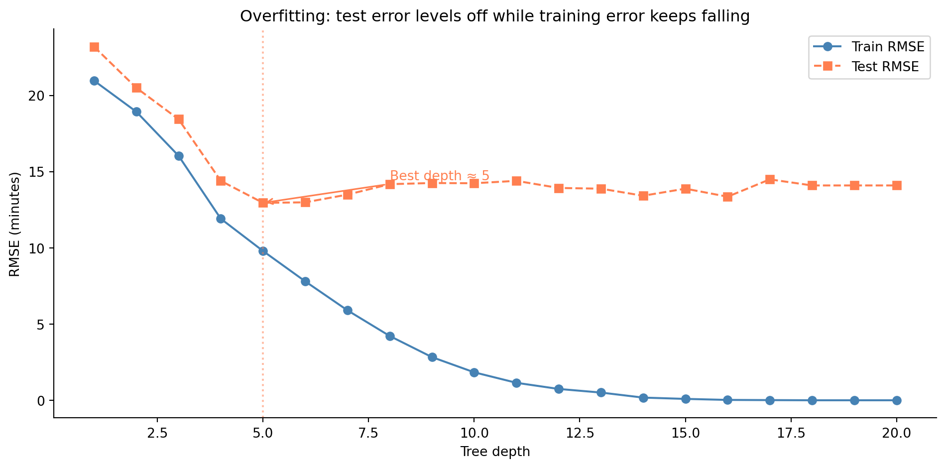
#| fig-cap: "Train and test RMSE across tree depths. Training error drops to near zero, but test error levels off after depth 5–7 and fluctuates — the tree is fitting noise rather than signal."
#| fig-alt: "Line chart with tree depth on the horizontal axis and RMSE on the vertical axis. The blue training error line with circle markers decreases steadily from about 12 at depth 1 to near 0 at depth 15. The orange test error line with square markers decreases until around depth 5–7, then levels off and fluctuates, with a vertical dashed annotation marking the approximate best depth."
depths = range(1, 21)
train_rmses, test_rmses = [], []

for d in depths:
    dt = DecisionTreeRegressor(max_depth=d, random_state=42)
    dt.fit(X_train, y_train)
    train_rmses.append(root_mean_squared_error(y_train, dt.predict(X_train)))
    test_rmses.append(root_mean_squared_error(y_test, dt.predict(X_test)))

best_depth = list(depths)[np.argmin(test_rmses)]

fig, ax = plt.subplots(figsize=(10, 5))
fig.patch.set_alpha(0)
ax.patch.set_alpha(0)
ax.plot(list(depths), train_rmses, 'o-', color='#0072B2', label='Train RMSE')
ax.plot(list(depths), test_rmses, 's--', color='#E69F00', label='Test RMSE')
ax.axvline(best_depth, color='#E69F00', linestyle=':', alpha=0.5)
ax.annotate(f'Best depth ≈ {best_depth}',
            xy=(best_depth, min(test_rmses)),
            xytext=(best_depth + 3, min(test_rmses) + 1.5),
            fontsize=10, color='#E69F00',
            arrowprops=dict(arrowstyle='->', color='#E69F00', lw=1.2))
ax.set_xlabel('Tree depth')
ax.set_ylabel('RMSE (minutes)')
ax.set_title('Overfitting: test error levels off while training error keeps falling')
ax.legend()
ax.spines[['top', 'right']].set_visible(False)
plt.tight_layout()
plt.show()
```
Compare this to the train/test error curves from @fig-train-test-error in the regularisation chapter. The pattern is the same in spirit: training error decreases as you add flexibility, but test error stops improving and may worsen. Beyond the optimal depth, the tree is learning noise rather than signal. Cross-validation (the same technique from @sec-choosing-alpha) is the principled way to choose the right depth.
## Random forests: the ensemble idea {#sec-random-forests}
A single decision tree is unstable. Train it on a slightly different sample and you might get a completely different set of splits, the same high-variance problem that plagued the high-degree polynomial. The insight behind **random forests** [@breiman2001rf] is disarmingly simple: if one tree is unreliable, train many trees and average their predictions.
The mechanism has two parts. **Bagging** (bootstrap aggregating) trains each tree on a different random sample drawn *with replacement* from the training data, meaning each observation can appear multiple times in a given sample. Each bootstrap sample is the same size as the original but contains some observations multiple times and omits others entirely. This means each tree sees a slightly different view of the data, and their individual errors tend to cancel out when averaged.
**Feature randomisation** adds a second layer of diversity. At each split, instead of considering all features, the tree only considers a random subset. The standard recommendation is $\sqrt{p}$ features for classification or $p/3$ for regression, where $p$ denotes the number of features (not a proportion). Note that scikit-learn's defaults differ from these recommendations: `RandomForestClassifier` defaults to $\sqrt{p}$, but `RandomForestRegressor` defaults to using *all* features. To follow the literature recommendation, set `max_features` explicitly. This feature subsetting prevents every tree from splitting on the same dominant feature first, producing trees that are decorrelated — they make different mistakes, which is exactly what you want when averaging.
An elegant side effect of bagging: each tree sees roughly $1 - 1/e \approx 63.2\%$ of the training data, leaving roughly $1/e \approx 36.8\%$ unseen. These unseen observations — the **out-of-bag** (OOB) samples — form a natural validation set for that tree. The average prediction error across the OOB samples gives an honest estimate of test-set performance without needing a separate holdout set.
```{python}
#| label: random-forest-fit
#| echo: true
from sklearn.ensemble import RandomForestRegressor

rf = RandomForestRegressor(
    n_estimators=200, random_state=42, oob_score=True, n_jobs=-1
)
rf.fit(X_train, y_train)

rf_test_rmse = root_mean_squared_error(y_test, rf.predict(X_test))
rf_train_rmse = root_mean_squared_error(y_train, rf.predict(X_train))

print("Random forest (200 trees):")
print(f"  Train RMSE:  {rf_train_rmse:.1f} min")
print(f"  Test RMSE:   {rf_test_rmse:.1f} min")
print(f"  OOB R²:      {rf.oob_score_:.3f}")
```
```{python}
#| label: fig-feature-importance
#| echo: true
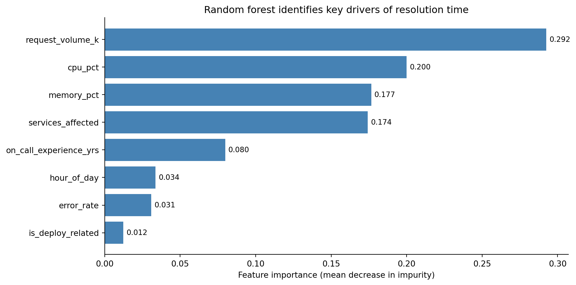
#| fig-cap: "Feature importance from the random forest, measured by mean decrease in impurity. The high-signal features our data-generating process made important — request volume, both resource-pressure metrics (CPU and memory), and services affected — dominate the top of the chart, while the low-signal features fall to the bottom."
#| fig-alt: "Horizontal bar chart showing feature importance for eight features. The high-signal features — request volume, CPU and memory pressure, and services affected — form the longest bars at the top, while the low-signal features (on-call experience, hour of day, error rate, and whether the incident was deploy-related) form much shorter bars at the bottom. Numeric values are labelled at the end of each bar. All bars are blue with no edge colour."
importances = rf.feature_importances_
sorted_idx = np.argsort(importances)

fig, ax = plt.subplots(figsize=(10, 5))
fig.patch.set_alpha(0)
ax.patch.set_alpha(0)
ax.barh(range(len(feature_names)), importances[sorted_idx],
        color='#0072B2', edgecolor='none')
ax.set_yticks(range(len(feature_names)))
ax.set_yticklabels(np.array(feature_names)[sorted_idx])
ax.set_xlabel('Feature importance (mean decrease in impurity)')
ax.set_title('Random forest identifies key drivers of resolution time')
ax.spines[['top', 'right']].set_visible(False)

for i, v in enumerate(importances[sorted_idx]):
    ax.text(v + 0.002, i, f'{v:.3f}', va='center', fontsize=9)

plt.tight_layout()
plt.show()
```
A word of caution on feature importance. The default "mean decrease in impurity" measure has known biases: it favours high-cardinality features (continuous variables with many possible split points get more opportunities to appear useful) and can be misleading when features are correlated. **Permutation importance**, which measures how much the model's accuracy degrades when a feature's values are randomly shuffled, is a more honest alternative, though slower to compute.
```{python}
#| label: permutation-importance
#| echo: true
from sklearn.inspection import permutation_importance

perm_imp = permutation_importance(rf, X_test, y_test, n_repeats=10, random_state=42)

print('Permutation importance (test set):')
perm_sorted = np.argsort(perm_imp.importances_mean)
for idx in perm_sorted[::-1]:
    print(f"  {feature_names[idx]:28s}: "
          f"{perm_imp.importances_mean[idx]:.3f} "
          f"± {perm_imp.importances_std[idx]:.3f}")
```
For a quick ranking during exploration, impurity-based importance is fine; for any decision that matters, verify with permutation importance.
::: {.callout-tip}
## Author's Note
The idea that averaging many *unreliable* models produces a *reliable* one sits in tension with engineering intuition. In a distributed system, running three replicas of a buggy service doesn't fix the bug: they'll all return the same wrong answer. The key difference is that replicas share the same code, whereas trees trained on bootstrap samples with random feature subsets make *different* mistakes. Averaging errors that point in different directions cancels them out. The closest engineering parallel is consensus in distributed systems: each node has an incomplete view of the cluster state, but the majority vote is more reliable than any individual node's opinion. The mechanism is identical: uncorrelated errors cancel. Bagging and feature randomisation are the mechanisms that guarantee the errors remain uncorrelated; without them, you'd just have many copies of the same mistake.
:::
## Gradient boosting: learning from mistakes {#sec-gradient-boosting}
Random forests build trees independently and average them. **Gradient boosting** takes a fundamentally different approach: it builds trees *sequentially*, where each new tree focuses on correcting the mistakes of the previous ensemble.
The process works like this. Start with a simple prediction: the mean of the training data. Compute the residuals (the gaps between predictions and actual values). Train a small tree to predict those residuals. Add that tree's predictions to the ensemble, scaled down by a **learning rate**, denoted $\eta$ (eta), which controls how much each tree contributes. Compute the new residuals and repeat.
Formally, after $m$ rounds:
$$
F_m(x) = F_{m-1}(x) + \eta \cdot h_m(x)
$$
where $F_{m-1}$ is the ensemble so far, $h_m$ is the new tree fitted to the current residuals, and $\eta \in (0, 1]$ is the learning rate (also called **shrinkage**). Smaller values mean slower learning but better generalisation, because the ensemble takes many small corrective steps rather than a few large ones. For squared-error loss, the negative gradient equals the residuals, so each tree directly corrects the previous errors. For other loss functions (such as absolute error or log-loss for classification), the trees fit the negative gradient of the loss, a generalisation of the residual idea.
::: {.callout-note}
## Engineering Bridge
Gradient boosting is iterative refinement — the same workflow you use when debugging a complex system. You deploy, observe what's still wrong (the residuals), make a targeted fix (the next tree), and repeat. The learning rate is analogous to a damping coefficient in a control loop: each correction nudges the system towards the target but deliberately undershoots. If you've ever tuned a system where aggressive corrections cause oscillation while conservative ones converge slowly but stably, you've dealt with exactly this trade-off. A learning rate of 0.1 means each tree corrects only 10% of the remaining error — conservative, but the cumulative effect of many small corrections converges to an excellent model.
:::
The relationship between the learning rate and the number of trees involves a trade-off. A small learning rate needs more trees to converge but typically produces better results; a large learning rate converges faster but risks overshooting. In practice, set the learning rate to a small value (0.05–0.1) and increase `n_estimators` until the validation error stops improving.
Libraries like XGBoost and LightGBM provide highly optimised implementations with additional features (histogram-based splitting, regularisation, GPU support), but for understanding the core idea, scikit-learn's `GradientBoostingRegressor` is clearer and perfectly adequate for datasets of this size.
```{python}
#| label: gradient-boosting-fit
#| echo: true
from sklearn.ensemble import GradientBoostingRegressor

gb = GradientBoostingRegressor(
    n_estimators=200, learning_rate=0.1, max_depth=4, random_state=42
)
gb.fit(X_train, y_train)

gb_test_rmse = root_mean_squared_error(y_test, gb.predict(X_test))
gb_train_rmse = root_mean_squared_error(y_train, gb.predict(X_train))

print("Gradient boosting (200 trees, lr=0.1, depth=4):")
print(f"  Train RMSE: {gb_train_rmse:.1f} min")
print(f"  Test RMSE:  {gb_test_rmse:.1f} min")

# Compare all models so far
for model_name, rmse in [('Linear regression', lr_test_rmse),
                          ('Decision tree (depth 3)', dt_test_rmse),
                          ('Random forest (200)', rf_test_rmse),
                          ('Gradient boosting (200)', gb_test_rmse)]:
    print(f"  {model_name}: {rmse:.1f} min")
```
```{python}
#| label: fig-staged-predictions
#| echo: true
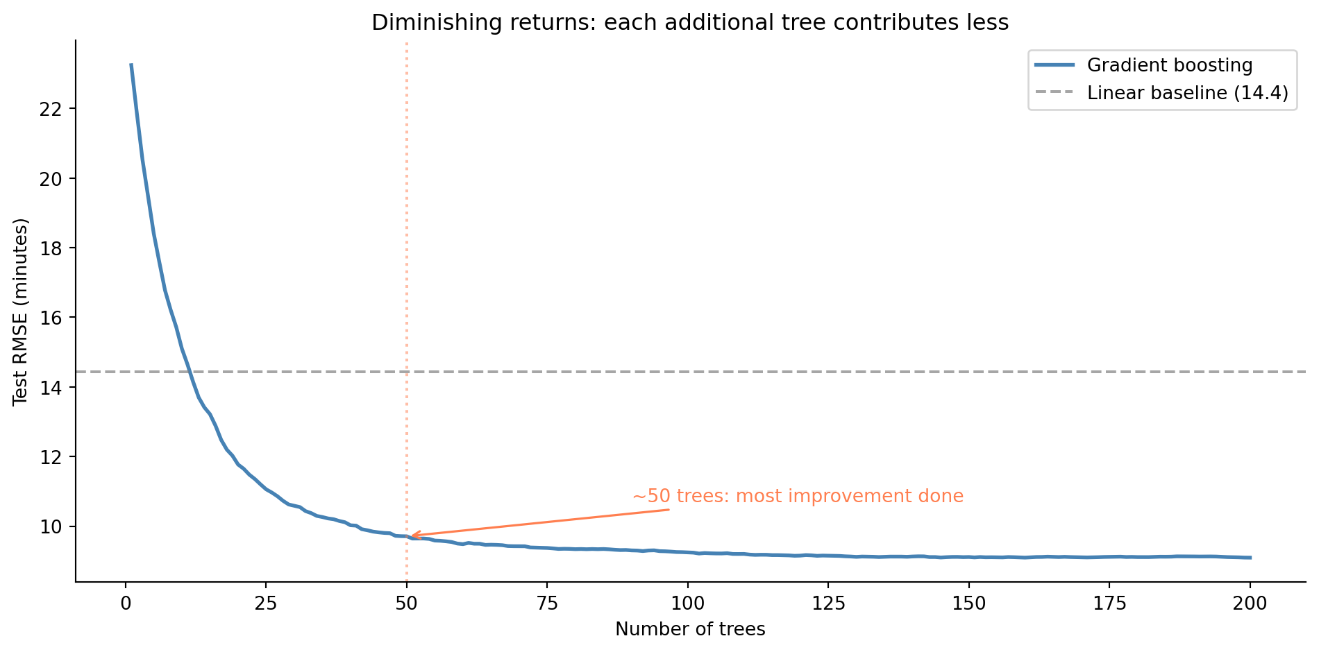
#| fig-cap: "Test RMSE as gradient boosting adds trees. Error drops steeply in the first 50 trees, then gradually levels off. The linear baseline is shown for reference."
#| fig-alt: "Line chart with number of trees on the horizontal axis and test RMSE on the vertical axis. The blue line drops steeply from about 23 minutes at 1 tree to about 10 minutes at 50 trees, then gradually levels off around 9 minutes by 200 trees. A horizontal grey dashed line marks the linear regression baseline at a higher RMSE. A vertical orange dotted line marks approximately 50 trees where diminishing returns begin."
# Staged predictions show the learning curve
staged_rmses = []
for y_staged in gb.staged_predict(X_test):
    staged_rmses.append(root_mean_squared_error(y_test, y_staged))

fig, ax = plt.subplots(figsize=(10, 5))
fig.patch.set_alpha(0)
ax.patch.set_alpha(0)
ax.plot(range(1, len(staged_rmses) + 1), staged_rmses, color='#0072B2',
        linewidth=2, label='Gradient boosting')
ax.axhline(lr_test_rmse, color='grey', linestyle='--', alpha=0.7,
           label=f'Linear baseline ({lr_test_rmse:.1f})')
ax.axvline(50, color='#E69F00', linestyle=':', alpha=0.5)
ax.annotate('~50 trees: most improvement done',
            xy=(50, staged_rmses[49]),
            xytext=(90, staged_rmses[49] + 1),
            fontsize=10, color='#E69F00',
            arrowprops=dict(arrowstyle='->', color='#E69F00', lw=1.2))
ax.set_xlabel('Number of trees')
ax.set_ylabel('Test RMSE (minutes)')
ax.set_title('Diminishing returns: each additional tree contributes less')
ax.legend()
ax.spines[['top', 'right']].set_visible(False)
plt.tight_layout()
plt.show()
```
The staged prediction plot reveals how boosting works: each additional tree chips away at the error, with diminishing returns. The first 50 trees do most of the work: they capture the dominant patterns. The remaining trees provide incremental refinement. This is the sequential correction process in action: early trees fix the big misses, later trees fine-tune.
## Trees for classification {#sec-tree-classification}
Everything we've built so far predicts a continuous outcome, resolution time in minutes. But the same tree-based models work for classification with minimal changes. The splitting criterion shifts from variance reduction to **Gini impurity**. For a node with $K$ classes where class $k$ has proportion $p_k$:
$$
G = 1 - \sum_{k=1}^{K} p_k^2
$$
In words, Gini impurity equals one minus the sum of the squared class proportions. It is zero when a node is pure (all observations belong to one class) and reaches its maximum when classes are equally mixed. You can think of it as the probability that two randomly chosen observations from the node would have different classes. A split is good if it produces children with lower Gini impurity, meaning more homogeneous groups.
```{python}
#| label: gini-calculation
#| echo: true
# Gini impurity: quick computation
def gini(proportions):
    return 1 - sum(p ** 2 for p in proportions)

# A pure node (all one class): Gini = 0
print(f"Pure node [1.0, 0.0]:    Gini = {gini([1.0, 0.0]):.2f}")
# Maximally mixed: Gini = 0.5 for binary
print(f"Mixed node [0.5, 0.5]:   Gini = {gini([0.5, 0.5]):.2f}")
# Somewhat mixed
print(f"Partial [0.8, 0.2]:      Gini = {gini([0.8, 0.2]):.2f}")
```
The prediction at each leaf becomes a class label (or probability) rather than a mean. Let's derive a classification target from our incident data. An incident is *critical* if it takes more than 55 minutes to resolve; these are the incidents that need immediate escalation.
```{python}
#| label: fig-classification-auc
#| echo: true
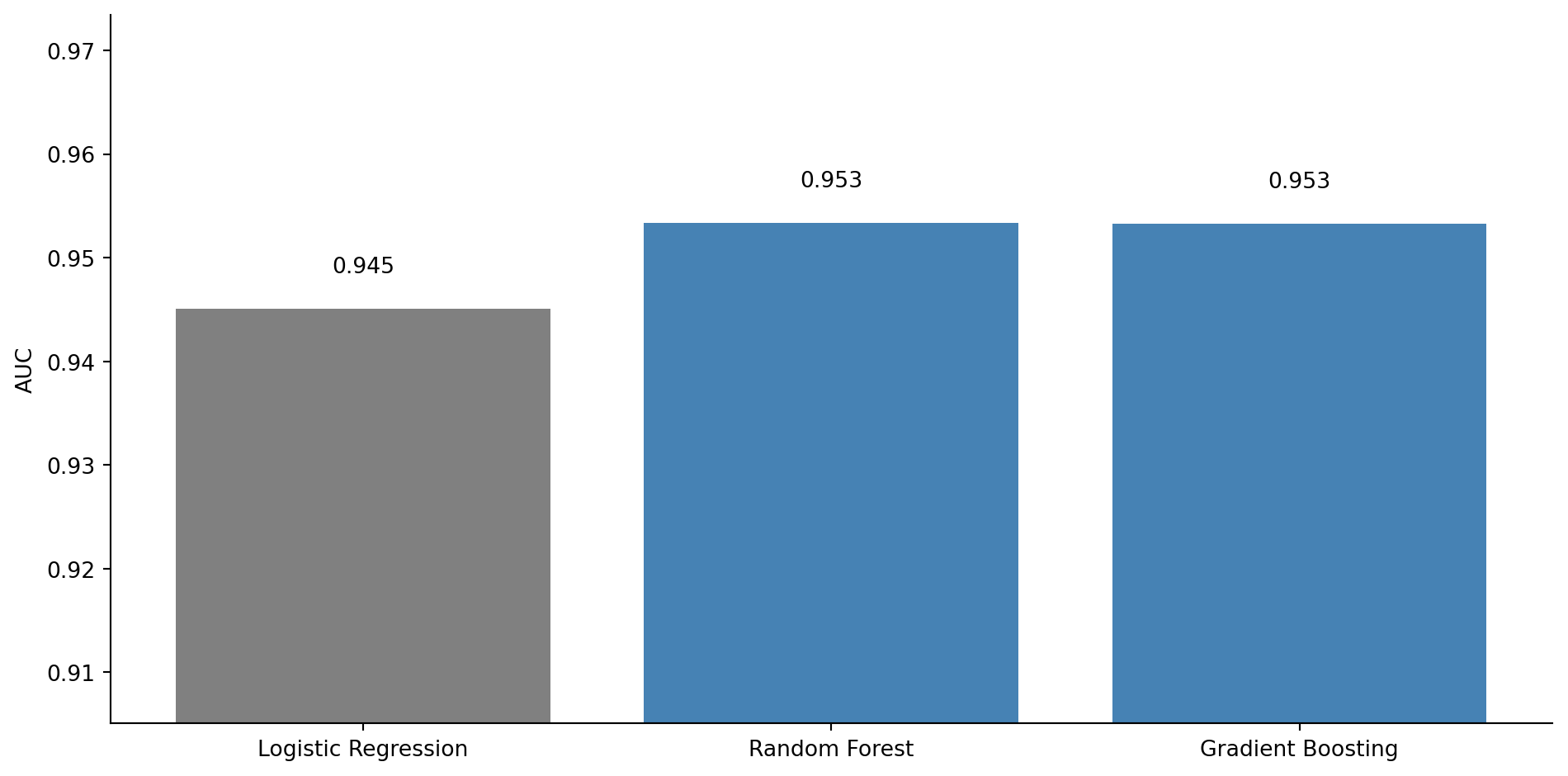
#| fig-cap: "AUC (area under the ROC curve) comparison across classifiers. The grey bar shows logistic regression; the blue bars show ensemble methods. All three models achieve high AUC (above 0.9), with the tree-based ensembles edging ahead — read the numeric labels rather than the bar heights to gauge the differences."
#| fig-alt: "Bar chart comparing AUC scores for three classifiers. Logistic Regression has the shortest bar at approximately 0.94, Random Forest is taller at approximately 0.95, and Gradient Boosting is tallest at approximately 0.95. AUC values are labelled above each bar. The logistic regression bar is grey; the two ensemble bars are blue."
from sklearn.linear_model import LogisticRegression
from sklearn.ensemble import RandomForestClassifier, GradientBoostingClassifier
from sklearn.metrics import roc_auc_score

# Derive binary classification target
y_critical = (y > 55).astype(int)
y_train_cls = y_critical.loc[X_train.index]
y_test_cls = y_critical.loc[X_test.index]

print(f"Critical incident rate: {y_critical.mean():.1%}")

classifiers = {
    'Logistic Regression': LogisticRegression(max_iter=200, random_state=42),
    'Random Forest': RandomForestClassifier(
        n_estimators=200, random_state=42, n_jobs=-1
    ),
    'Gradient Boosting': GradientBoostingClassifier(
        n_estimators=200, learning_rate=0.1, max_depth=4, random_state=42
    ),
}

auc_scores = {}
for name, clf in classifiers.items():
    clf.fit(X_train, y_train_cls)
    y_prob = clf.predict_proba(X_test)[:, 1]
    auc_scores[name] = roc_auc_score(y_test_cls, y_prob)

fig, ax = plt.subplots(figsize=(10, 5))
fig.patch.set_alpha(0)
ax.patch.set_alpha(0)
names = list(auc_scores.keys())
aucs = list(auc_scores.values())
bar_colours = ['grey', '#0072B2', '#0072B2']
bars = ax.bar(names, aucs, color=bar_colours, edgecolor='none')
bars[0].set_hatch('//')  # distinguish the linear baseline

for bar, auc_val in zip(bars, aucs):
    ax.text(bar.get_x() + bar.get_width() / 2, bar.get_height() + 0.003,
            f'{auc_val:.3f}', ha='center', va='bottom', fontsize=10)

ax.set_ylabel('AUC')
ax.set_ylim(0, 1.05)
ax.spines[['top', 'right']].set_visible(False)
plt.tight_layout()
plt.show()
```
All three models perform well: logistic regression achieves an AUC above 0.9, which is strong. The tree-based ensemble methods edge ahead because they can capture the non-linear interactions (the CPU-memory spike, the request volume threshold) more precisely. The gap is modest because collapsing resolution time to a binary outcome substantially linearises the original non-linear relationships: the step functions in the data-generating process become easier to approximate with a linear decision boundary in eight-dimensional feature space.
AUC is a useful single number, but it averages over every possible threshold. To see *what kind* of mistakes the random forest is actually making at the default threshold of 0.5, look at the confusion matrix.
```{python}
#| label: fig-tree-confusion-matrix
#| echo: true
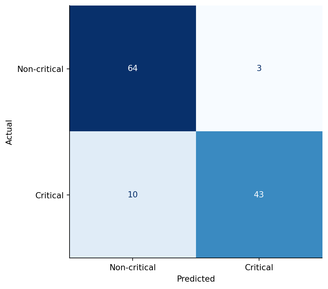
#| fig-cap: "Random forest confusion matrix on the critical-incident classification. Rows are the true class, columns are the predicted class. The diagonal counts correct predictions; the off-diagonal cells separate false positives (top-right) from false negatives (bottom-left)."
#| fig-alt: "Two-by-two heatmap. Rows labelled Non-critical and Critical (true); columns labelled Non-critical and Critical (predicted). The diagonal cells are darker, showing the bulk of correct predictions. The bottom-left cell (false negatives — missed critical incidents) and top-right cell (false positives — non-critical incidents flagged as critical) are visibly lighter."
from sklearn.metrics import confusion_matrix, ConfusionMatrixDisplay

rf_clf = classifiers['Random Forest']
y_pred_rf = rf_clf.predict(X_test)
cm = confusion_matrix(y_test_cls, y_pred_rf)

fig, ax = plt.subplots(figsize=(6, 5))
fig.patch.set_alpha(0)
ax.patch.set_alpha(0)
disp = ConfusionMatrixDisplay(cm, display_labels=['Non-critical', 'Critical'])
disp.plot(ax=ax, cmap='Blues', colorbar=False)
ax.set_xlabel('Predicted')
ax.set_ylabel('Actual')
plt.tight_layout()
plt.show()

tn, fp, fn, tp = cm.ravel()
print(f"Recall (critical caught): {tp / (tp + fn):.1%}")
print(f"Precision (alerts that were real): {tp / (tp + fp):.1%}")
```
Two observations. First, the false negatives — the critical incidents the model failed to flag — are the costly errors in this domain: a missed escalation means a long-running outage isn't surfaced to the on-call engineer. Second, the precision and recall numbers expose what the AUC bar chart hid: at the 0.5 threshold the random forest is conservative about declaring an incident critical. If the operational cost of a missed escalation outweighs the cost of a false alarm, lower the threshold and re-read the matrix. The same threshold-tuning calculus from @sec-roc-auc applies to tree-based classifiers without modification.
## When to use what {#sec-trees-vs-linear}
Tree-based models aren't universally superior. Each model family has strengths and weaknesses, and the choice depends on the problem.
| Criterion | Linear / Logistic | Decision Tree | RF / Boosting |
| --: | :-- | :-- | :-- |
| Interpretability | High (coefficients) | High (visualise the tree) | Low (black box) |
| Non-linear relationships | Manual (polynomials, transforms) | Automatic | Automatic |
| Feature interactions | Manual (interaction terms) | Automatic | Automatic |
| Needs feature scaling | Yes (for regularised) | No | No |
| Training speed (small data) | Fast | Fast | Slower |
| Handles missing values | No (impute first) | Yes (native in sklearn ≥ 1.3) | RF: Yes; GradientBoostingRegressor: No (use HistGradientBoostingRegressor) |
| Extrapolation | Reasonable | Poor (constant beyond data) | Poor (constant beyond data) |
| Sample size guidance | ~50–100 | ~100–200 | ~200–500 |
: Comparison of model families. Sample size values are rough heuristics that depend heavily on the signal-to-noise ratio and number of features — treat them as order-of-magnitude guidance, not hard thresholds. {#tbl-model-comparison}
Trees don't need feature scaling because they split on thresholds rather than computing weighted sums: they're invariant to monotonic transformations of the features (any transformation that preserves order, such as log or squaring positive values). Whether CPU is measured in percentage (0–100) or as a fraction (0–1), the tree finds the same splits. This is a genuine advantage over regularised linear models, which require standardisation as we saw in @sec-ridge.
Linear models extrapolate more gracefully, and this is the single biggest limitation of tree-based models. A tree's prediction outside the range of the training data is a constant, the mean of the nearest leaf. If your training incidents had CPU between 20% and 99%, a tree predicting for 100% CPU will give the same answer as for 99%. A linear model at least continues the trend, which may or may not be correct, but it's a more principled guess for modest extrapolation.
When the relationship really is linear, linear models are also the better choice. If the true data-generating process is $y = \beta_0 + \beta_1 x + \varepsilon$ — no interactions, no thresholds — a linear model captures this exactly with two parameters. A random forest needs hundreds of trees and thousands of splits to approximate a straight line. Trees shine when relationships are complex and you don't know the functional form in advance.
Finally, interpretability is a spectrum. A single decision tree is among the most interpretable models: you can literally read the rules. A random forest of 200 trees is effectively a black box. If your stakeholders need to understand *why* the model predicts what it does (regulatory requirements, debugging, trust-building), a single tree or linear model may be worth the accuracy trade-off.
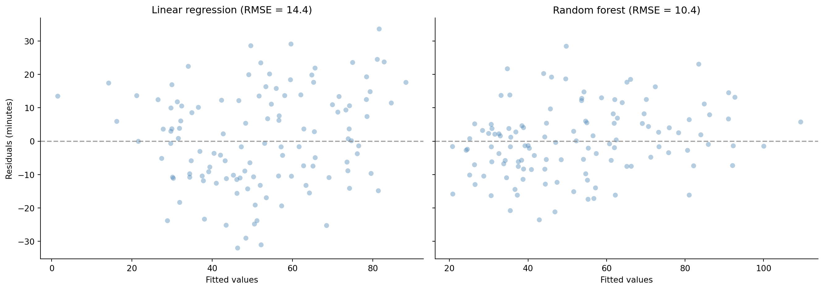
To close the loop visually, compare the residuals from the linear model (which opened this chapter) with those from the random forest:
```{python}
#| label: fig-residual-comparison
#| echo: true
#| fig-cap: "Residuals from the linear model (left) show systematic curvature; residuals from the random forest (right) scatter randomly around zero. The non-linear patterns that the linear model missed have been captured."
#| fig-alt: "Two-panel scatter plot. Left panel shows linear regression residuals versus fitted values with a clear curved pattern indicating model misspecification. Right panel shows random forest residuals versus fitted values with no discernible pattern, scattered randomly around the zero line. Both panels use blue points and a horizontal grey dashed reference line at zero."
fig, (ax1, ax2) = plt.subplots(1, 2, figsize=(14, 5), sharey=True)
fig.patch.set_alpha(0)
ax1.patch.set_alpha(0)
ax2.patch.set_alpha(0)

# Linear residuals
lr_resid = y_test - lr.predict(X_test)
ax1.scatter(lr.predict(X_test), lr_resid, alpha=0.4, color='#0072B2',
            edgecolor='none')
ax1.axhline(0, color='grey', linestyle='--', alpha=0.7)
ax1.set_xlabel('Fitted values')
ax1.set_ylabel('Residuals (minutes)')
ax1.set_title(f'Linear regression (RMSE = {lr_test_rmse:.1f})')
ax1.spines[['top', 'right']].set_visible(False)

# Random forest residuals
rf_resid = y_test - rf.predict(X_test)
ax2.scatter(rf.predict(X_test), rf_resid, alpha=0.4, color='#0072B2',
            edgecolor='none')
ax2.axhline(0, color='grey', linestyle='--', alpha=0.7)
ax2.set_xlabel('Fitted values')
ax2.set_title(f'Random forest (RMSE = {rf_test_rmse:.1f})')
ax2.spines[['top', 'right']].set_visible(False)

plt.tight_layout()
plt.show()
```
## Summary {#sec-tree-models-summary}
1. **Decision trees partition the feature space through recursive binary splits**, learning if-else rules from data. They handle non-linearity and feature interactions naturally, without manual feature engineering.
2. **Unrestricted trees overfit** by memorising the training data. Controlling depth, minimum leaf size, or cost-complexity pruning manages the bias-variance trade-off — the same principle from @sec-bias-variance applied to a different model family.
3. **Random forests reduce variance by averaging many decorrelated trees**, each trained on a bootstrap sample with random feature subsets. Out-of-bag error provides a free validation estimate.
4. **Gradient boosting reduces bias by building trees sequentially**, each correcting the residuals of the previous ensemble. The learning rate controls the step size, trading convergence speed for generalisation.
5. **Tree-based models don't need feature scaling and handle interactions automatically**, but they extrapolate poorly and sacrifice interpretability (in ensemble form). Linear models remain better when relationships are truly linear or when interpretability is paramount.
## Exercises {#sec-tree-models-exercises}
1. Using the incident data from this chapter, fit `DecisionTreeRegressor` at depths 2, 5, and 10. Visualise each tree using `plot_tree` and report test RMSE. At what depth does the tree start to overfit? What splits does the depth-2 tree discover?
2. Use `DecisionTreeRegressor` with `cost_complexity_pruning_path` to find the optimal `ccp_alpha` via 5-fold cross-validation. Compare the pruned tree's test RMSE to the depth-limited trees from Exercise 1. How many leaves does the optimal pruned tree have?
3. Plot the random forest's OOB score (set `oob_score=True` and `warm_start=True`) as `n_estimators` increases from 10 to 500. At what point do additional trees stop meaningfully improving the OOB score?
4. **Conceptual:** We compared a decision tree to a learned if-else chain. Where does this analogy break down? Think specifically about how a tree handles data it has never seen before (extrapolation) compared to hand-coded dispatch logic. What kinds of inputs would expose this limitation?
5. **Conceptual:** Random forests reduce variance by averaging (many independent estimates produce a more stable result). Gradient boosting reduces bias by sequential correction (each step fixes the previous step's mistakes). Explain intuitively why *averaging* helps with variance and *sequential fitting* helps with bias. Can you think of an engineering workflow that mirrors each strategy?