---
# Content: CC BY-NC-SA 4.0 | Code: MIT - see /LICENSE.md
title: "Bayesian inference: updating beliefs with evidence"
---
{{< include /_common-imports.qmd >}}
## From fixed parameters to uncertain beliefs {#sec-bayesian-inference}
Throughout Part 2, we've been asking questions of the form "is the data surprising, assuming $H_0$ is true?" The p-value answers this, but it answers a *different* question from the one you actually need answered: "given this data, how likely is the hypothesis?"
In @sec-p-value-pitfalls, we flagged this distinction: $P(\text{data} \mid H_0)$ is not the same as $P(H_0 \mid \text{data})$. In @sec-bayes, we saw Bayes' theorem as a rule for updating probabilities. This chapter takes that rule and turns it into a full inference framework, one where parameters aren't fixed unknowns to be estimated, but uncertain quantities with probability distributions of their own.
The shift is conceptual, not mathematical. In frequentist inference, the conversion rate $p$ *has* a true value; we just don't know it. In Bayesian inference, we model our uncertainty about $p$ as a probability distribution, a random variable whose spread reflects how much we know. Observing data narrows that distribution. The generic symbol for such a parameter is $\theta$ (theta); we'll use it throughout this chapter whenever we're talking about an unknown quantity in general, and switch to $p$ when the parameter is specifically a proportion.
If you've ever updated a rolling estimate — adjusting your belief about system latency as new metrics arrive, or revising a project timeline as tasks complete — you've been thinking like a Bayesian. This chapter formalises that instinct.
## The Bayesian recipe {#sec-bayesian-recipe}
Every Bayesian analysis follows three steps, each feeding into the next. First, you choose a **prior** $P(\theta)$: what you believe about the parameter before seeing data. This can be vague ("any value between 0 and 1 is equally likely") or informative ("based on past experiments, the conversion rate is around 12%"). Second, you compute the **likelihood** $P(\text{data} \mid \theta)$: how probable the observed data is for each possible value of $\theta$. This is the same likelihood that underlies maximum likelihood estimation (MLE, finding the parameter value that makes the observed data most probable) and hypothesis tests. Third, you apply **Bayes' theorem** to combine the prior and likelihood into the **posterior** $P(\theta \mid \text{data})$: your updated belief after seeing the data.
$$
P(\theta \mid \text{data}) = \frac{P(\text{data} \mid \theta) \times P(\theta)}{P(\text{data})}
$$
The denominator $P(\text{data})$ is a normalising constant, a scaling factor that ensures the posterior is a valid probability distribution (its total area equals 1). For most practical problems, you don't compute it directly; the shape of the posterior is determined entirely by the numerator.
In plain language: **posterior $\propto$ likelihood $\times$ prior** (where $\propto$ means "is proportional to", equal up to a constant scaling factor). Your updated belief is proportional to the data's support for each parameter value, weighted by what you believed beforehand.
To model a prior over a proportion (a value between 0 and 1), we use the **Beta distribution**, a continuous distribution parameterised by two shape parameters, conventionally written $\alpha$ and $\beta$. (Don't confuse this $\alpha$ with the significance level from hypothesis testing, or this $\beta$ with the Type II error rate; both are unfortunate but standard collisions. Context makes clear which is meant.)
The Beta distribution wasn't in our original distribution toolkit (@sec-distribution-tour), but it earns its place here because it is the natural distribution for uncertain proportions. When $\alpha = \beta = 1$, it reduces to a Uniform(0, 1); when both are greater than 1, it forms a hump centred near $\alpha / (\alpha + \beta)$. In scipy, it lives at `stats.beta(a, b)`.
```{python}
#| label: fig-bayesian-grid
#| echo: true
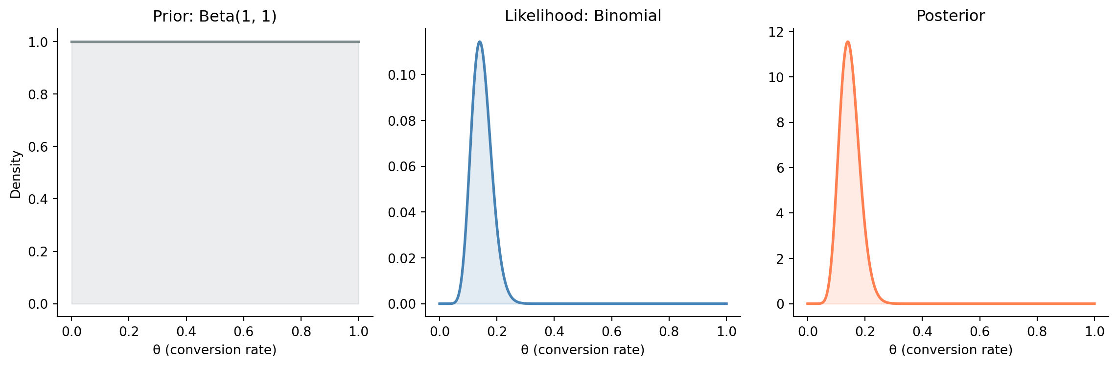
#| fig-cap: "The Bayesian recipe applied to a conversion rate problem. A uniform prior (left) combined with the binomial likelihood for 14 conversions in 100 visitors (centre) produces a posterior concentrated around 0.14 (right)."
#| fig-alt: "Three-panel figure. Left: a flat horizontal line showing the uniform Beta(1,1) prior density. Centre: a peaked binomial likelihood curve centred near 0.14. Right: the resulting posterior distribution, also peaked near 0.14, showing that with a uniform prior the posterior is dominated by the data."
from scipy import stats

# A website had 14 conversions out of 100 visitors.
# What is the conversion rate? (theta here *is* the conversion rate —
# we use the generic symbol because the Bayesian machinery works for any parameter.)
n_obs = 100
k_obs = 14

# Step 1: Prior — Beta(1, 1) is uniform on [0, 1]:
# "any conversion rate is equally plausible."
theta = np.linspace(0, 1, 1000)
prior = stats.beta.pdf(theta, 1, 1)

# Step 2: Likelihood — same binom.pmf we used for binomial distributions, but differently.
# There we fixed p and asked "what's the probability of k successes?"
# Here we fix the data (k=14, n=100) and ask "how probable is this data
# for each candidate theta?" — this is the **likelihood function**.
# Note: as a function of theta this is unnormalised (its area need not equal 1),
# which is why only the posterior panel is a true density and the y-scales differ.
likelihood = stats.binom.pmf(k_obs, n_obs, theta)

# Step 3: Posterior is proportional to likelihood × prior
unnormalised_posterior = likelihood * prior
# Numerical integration (trapezoidal rule) — ensures the posterior integrates to 1
posterior = unnormalised_posterior / np.trapezoid(unnormalised_posterior, theta)

fig, axes = plt.subplots(1, 3, figsize=(12, 4), sharey=False)
fig.patch.set_alpha(0)

for ax, y, title, colour in zip(
    axes,
    [prior, likelihood, posterior],
    ['Prior\n(before data)', 'Likelihood\n(data evidence)', 'Posterior\n(after data)'],
    ['#7f8c8d', '#0072B2', '#E69F00'],
):
    ax.patch.set_alpha(0)
    ax.plot(theta, y, color=colour, linewidth=2)
    ax.fill_between(theta, y, alpha=0.25, color=colour)
    ax.set_title(title)
    ax.set_xlabel('θ (conversion rate)')
    ax.spines[['top', 'right']].set_visible(False)

axes[0].set_ylabel('Density')
plt.tight_layout()
plt.show()
```
@fig-bayesian-grid shows the result. With a uniform prior, the posterior is entirely driven by the data. The peak sits at 0.14 (the observed conversion rate), and the spread reflects our uncertainty given 100 observations. More data would narrow the posterior further; uncertainty shrinks as evidence accumulates.
## Conjugate priors: analytical shortcuts {#sec-conjugate-priors}
In the example above, we computed the posterior on a grid: evaluating the prior and likelihood at 1,000 candidate values of $\theta$, then normalising. This brute-force approach works for one parameter, but scales poorly to models with many parameters.
Fortunately, certain prior–likelihood pairings produce posteriors that have a known closed-form distribution (an explicit formula rather than a numerical approximation). These are called **conjugate priors**. The most useful one for binary data:
| Data model | Conjugate prior | Posterior |
|:------------------------|:-----------------------|:-----------------------------------|
| Binomial$(n, \theta)$ | Beta$(\alpha, \beta)$ | Beta$(\alpha + k, \beta + n - k)$ |
: The Beta–Binomial conjugate pair. {#tbl-conjugate}
If your prior is $\text{Beta}(\alpha, \beta)$ and you observe $k$ successes in $n$ trials, the posterior is $\text{Beta}(\alpha + k, \beta + n - k)$. No grid, no numerical integration — just add the counts to the prior parameters.
```{python}
#| label: conjugate-update
#| echo: true
# Prior: Beta(1, 1) — uniform
alpha_prior, beta_prior = 1, 1

# Data: 14 conversions out of 100
k, n = 14, 100

# Posterior: Beta(1 + 14, 1 + 86) = Beta(15, 87)
alpha_post = alpha_prior + k
beta_post = beta_prior + (n - k)

posterior_dist = stats.beta(alpha_post, beta_post)

print(f"Prior:     Beta({alpha_prior}, {beta_prior})")
print(f"Data:      {k} successes in {n} trials")
print(f"Posterior: Beta({alpha_post}, {beta_post})")
print(f"\nPosterior mean:   {posterior_dist.mean():.4f}")
print(f"Posterior median: {posterior_dist.median():.4f}")
# Beta mode = (α-1)/(α+β-2); only defined when α,β > 1
print(f"Posterior mode:   {(alpha_post - 1) / (alpha_post + beta_post - 2):.4f}")

# 95% credible interval: take the 2.5th and 97.5th percentiles of the posterior.
# ppf = percent point function (inverse CDF): ppf(0.025) gives the value below
# which 2.5% of the posterior mass falls. Same idea as CI construction,
# but applied to the posterior distribution rather than the sampling distribution.
cri_lower, cri_upper = posterior_dist.ppf(0.025), posterior_dist.ppf(0.975)
print(f"95% credible interval: ({cri_lower:.4f}, {cri_upper:.4f})")
```
The prior parameters $\alpha$ and $\beta$ in a Beta distribution can be interpreted as **pseudo-counts**, imaginary prior observations. Beta$(1, 1)$ acts as though you've seen 1 success and 1 failure before collecting any real data; Beta$(5, 45)$ is like starting with 5 successes in 50 trials, a prior belief centred on 10%. The data then adds its counts on top. (This pseudo-count interpretation matches the posterior mean formula $\alpha / (\alpha + \beta)$. The posterior mode uses $(\alpha - 1) / (\alpha + \beta - 2)$ for $\alpha, \beta > 1$. The uniform prior is a special case: because every value is equally plausible, the posterior is shaped entirely by the likelihood, and the posterior mode coincides exactly with the MLE. This is why maximum likelihood estimation can be understood as Bayesian MAP estimation with a uniform prior.)
This interpretation makes the prior tangible: you can ask "how many observations is my prior worth?" and compare that to the actual sample size. A Beta$(1, 1)$ prior is worth 2 pseudo-observations, negligible compared to 100 real ones, which is why the posterior is dominated by the data. A Beta$(50, 450)$ prior is worth 500 pseudo-observations and would take substantial data to overwhelm.
## Credible intervals: saying what you mean {#sec-credible-intervals}
In @sec-confidence-intervals, we built confidence intervals, ranges that, across repeated sampling, would contain the true parameter 95% of the time. The Bayesian equivalent is simpler to state and interpret.
A **95% credible interval** contains the parameter with 95% probability, given the data and the prior. No hypothetical repetitions, no tortured "if we repeated this procedure many times" language. The posterior *is* the distribution of the parameter, so we just read off the interval that captures 95% of its probability mass. The most common approach (and the one we use throughout this chapter) takes the 2.5th and 97.5th percentiles, giving an **equal-tailed** credible interval. (An alternative, the **highest posterior density** interval, finds the narrowest region containing 95% of the mass. For roughly symmetric posteriors, the two are nearly identical.)
```{python}
#| label: fig-credible-vs-confidence
#| echo: true
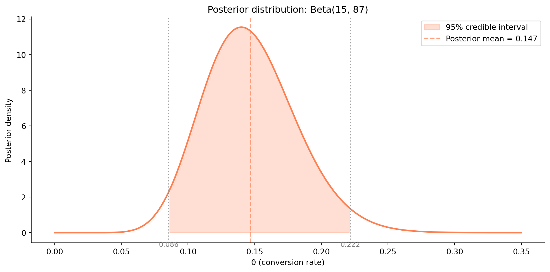
#| fig-cap: "Bayesian credible interval for the conversion rate. The shaded region contains 95% of the posterior probability mass — there is a 95% probability that the true conversion rate lies in this range, given the data and the prior."
#| fig-alt: "A peaked posterior density curve (orange) over conversion rate values from 0 to 0.35. The region between approximately 0.086 and 0.222 is shaded, representing the 95% credible interval. A dashed vertical line marks the posterior mean near 0.147. Grey dotted lines mark the interval boundaries."
fig, ax = plt.subplots(figsize=(10, 5))
fig.patch.set_alpha(0)
ax.patch.set_alpha(0)

theta = np.linspace(0, 0.35, 500)
pdf = posterior_dist.pdf(theta)

ax.plot(theta, pdf, '#E69F00', linewidth=2)
ax.fill_between(theta, pdf, where=(theta >= cri_lower) & (theta <= cri_upper),
                alpha=0.25, color='#E69F00', label='95% credible interval')

ax.axvline(posterior_dist.mean(), color='#E69F00', linestyle='--', alpha=0.7,
           label=f'Posterior mean = {posterior_dist.mean():.3f}')
ax.axvline(cri_lower, color='#555', linestyle=':', alpha=0.7)
ax.axvline(cri_upper, color='#555', linestyle=':', alpha=0.7)

ax.annotate(f'{cri_lower:.3f}', xy=(cri_lower, 0), xytext=(0, -18),
            textcoords='offset points', ha='center', fontsize=9, color='#555')
ax.annotate(f'{cri_upper:.3f}', xy=(cri_upper, 0), xytext=(0, -18),
            textcoords='offset points', ha='center', fontsize=9, color='#555')

ax.set_xlabel('θ (conversion rate)')
ax.set_ylabel('Posterior density')
ax.set_title(f'The conversion rate lies between {cri_lower:.1%} and {cri_upper:.1%} '
             f'with 95% probability', fontsize=11)
ax.legend()
ax.spines[['top', 'right']].set_visible(False)
plt.tight_layout()
plt.show()
```
As @fig-credible-vs-confidence shows, the credible interval and confidence interval often give numerically similar results, especially with large samples and weak priors. The difference is philosophical but practically meaningful: the credible interval directly answers "where is the parameter?" rather than the CI's indirect "what range would capture the parameter in 95% of repeated experiments?"
::: {.callout-note}
## Engineering Bridge
The interpretive difference matters in practice. An engineer who says "I'm 95% confident the p99 latency is between 180ms and 220ms based on this week's data" is making a credible-interval-style statement, a direct claim about where the parameter sits. A confidence interval says something subtler: "if I repeated this measurement procedure many times, 95% of the resulting intervals would contain the true value." Both are useful, but the credible interval matches how engineers naturally think about uncertainty. The cost is that you need a prior (which, as we'll see, is a feature when you have domain knowledge).
:::
## The prior matters (and that's OK) {#sec-prior-choice}
The most common objection to Bayesian inference is that the prior is "subjective." This is true, and it's a feature, not a bug. The prior is where domain knowledge enters the analysis. Ignoring relevant prior information doesn't make your analysis objective — it makes it wasteful.
```{python}
#| label: fig-prior-sensitivity
#| echo: true
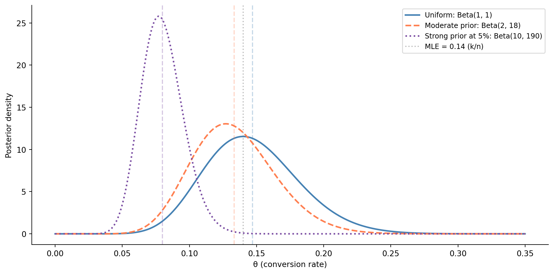
#| fig-cap: "Effect of different priors on the posterior, given the same data (14 conversions in 100 visitors). With enough data, the priors converge — but with limited data, the prior meaningfully shapes your conclusions."
#| fig-alt: "Line chart with three overlapping posterior density curves plotted against conversion rate from 0 to 0.35. The uniform prior (solid blue) and moderate prior (dashed orange) produce nearly identical posteriors peaked near 0.14. The strong prior centred at 5% (dotted purple) produces a visibly different posterior peaked near 0.08, demonstrating that with only 100 data points, a strong prior worth 200 pseudo-observations can materially shift conclusions. A grey dotted vertical line marks the MLE at 0.14."
fig, ax = plt.subplots(figsize=(10, 5))
fig.patch.set_alpha(0)
ax.patch.set_alpha(0)

theta = np.linspace(0, 0.35, 500)

priors = [
    ('Uniform: Beta(1, 1)', 1, 1, '#0072B2', '-'),
    ('Moderate prior: Beta(2, 18)', 2, 18, '#E69F00', '--'),
    ('Strong prior at 5%: Beta(10, 190)', 10, 190, '#CC79A7', ':'),
]

for label, a, b, colour, ls in priors:
    a_post = a + k
    b_post = b + (n - k)
    post = stats.beta(a_post, b_post)
    ax.plot(theta, post.pdf(theta), colour, linewidth=2, linestyle=ls, label=label)

ax.axvline(k / n, color='grey', linestyle=':', alpha=0.5,
           label=f'MLE = {k/n:.2f} (k/n)')  # the value that maximises the likelihood
ax.set_xlabel('θ (conversion rate)')
ax.set_ylabel('Posterior density')
ax.set_title('With 100 observations, only the strongest prior visibly shifts the estimate',
             fontsize=11)
ax.legend(fontsize=9)
ax.spines[['top', 'right']].set_visible(False)
plt.tight_layout()
plt.show()
```
@fig-prior-sensitivity illustrates the effect. With the uniform prior, the posterior mode equals the MLE (0.14); the data alone shapes the estimate. The moderate prior Beta$(2, 18)$, centred near 0.10 and worth 20 pseudo-observations, barely shifts the posterior given 100 real observations; the data dominates. The strong prior (equivalent to 200 pseudo-observations centred at 5%) is a different story: it pulls the posterior mean to approximately 0.08, well below the MLE. With 100 observations against 200 pseudo-observations of prior weight, the prior still has real influence.
The practical rule: **choose a prior that reflects genuine knowledge, not one designed to get the answer you want**. If you have no relevant prior information, use a weakly informative prior that regularises (constrains extreme estimates, much like adding a penalty to prevent overfitting) without dominating. If you have solid prior knowledge (from previous experiments, industry benchmarks, or domain constraints), encode it; that's information, and throwing it away has a cost.
::: {.callout-tip}
## Author's Note
The charge of subjectivity sounds damning until you notice that frequentist inference also rests on choices: the test, the significance level, the stopping rule, and the definition of "hypothetical repetitions" in a confidence interval are all decisions the analyst makes. The prior is not an additional source of subjectivity, it is just a more transparent one. Every analysis has assumptions; the Bayesian prior simply forces you to state yours explicitly rather than burying them in methodological defaults.
The practical response is a **sensitivity analysis**, repeating the analysis with different reasonable priors (as shown in @fig-prior-sensitivity) to check whether the conclusion changes. If it does, the data aren't strong enough to dominate, and you should say so. If it doesn't, the prior barely matters and the frequentist and Bayesian answers will agree.
:::
::: {.callout-tip}
## Author's Note
Engineers' first reaction to priors is often suspicion: "you're putting your thumb on the scale." That instinct is healthy, but it's pointed at the wrong problem. A prior isn't a bias toward a preferred conclusion; it operates like a regulariser — a constraint that prevents the estimate from chasing every fluctuation in a small sample. We'll meet regularisation directly in @sec-penalty-idea, but the engineering instinct is already familiar: you wouldn't deploy a 50-parameter model trained on 100 noisy observations without some form of penalty pulling the parameters toward something sensible. A prior does precisely that, at the inference layer rather than the optimisation layer. The Beta(8, 2) prior we use in the alerting example later in this chapter (@sec-bayesian-worked-example) is a gentle nudge of exactly this kind — worth only about ten pseudo-observations, so against a couple of hundred real alerts it lightly smooths the estimate rather than dominating it. Once you see priors as regularisers, the "subjectivity" objection becomes a milder engineering trade-off: how much do you trust the data alone, and how much smoothing do you want before you act?
:::
## Bayesian A/B testing {#sec-bayesian-ab}
The framework becomes especially powerful for the A/B testing problems we encountered in @sec-ab-testing. Instead of asking "is the difference statistically significant?", we can directly compute the probability that one variant is better than the other.
```{python}
#| label: bayesian-ab-test
#| echo: true
rng = np.random.default_rng(42)

# Observed data from an A/B test
n_control, n_variant = 4000, 4000
conversions_control = 480   # 12.0%
conversions_variant = 560   # 14.0%

# Uniform prior: Beta(1, 1) for both groups
alpha_prior, beta_prior = 1, 1

# Posterior distributions
posterior_control = stats.beta(
    alpha_prior + conversions_control,
    beta_prior + n_control - conversions_control
)
posterior_variant = stats.beta(
    alpha_prior + conversions_variant,
    beta_prior + n_variant - conversions_variant
)

# There's no simple formula for P(variant > control) when both are
# Beta-distributed, so we use **Monte Carlo simulation**: draw many
# random samples from each posterior and count how often variant wins.
n_samples = 100_000
samples_control = posterior_control.rvs(n_samples, random_state=rng)
samples_variant = posterior_variant.rvs(n_samples, random_state=rng)

p_variant_better = np.mean(samples_variant > samples_control)
lift_samples = samples_variant - samples_control

print(f"P(variant > control) = {p_variant_better:.4f}")
print(f"\nExpected lift: {np.mean(lift_samples):.4f} "
      f"({np.mean(lift_samples) * 100:.2f} percentage points)")
print(f"95% credible interval for lift: "
      f"({np.percentile(lift_samples, 2.5):.4f}, "
      f"{np.percentile(lift_samples, 97.5):.4f})")
print(f"\nP(lift > 1pp) = {np.mean(lift_samples > 0.01):.4f}")
print(f"P(lift > 2pp) = {np.mean(lift_samples > 0.02):.4f}")
```
This output directly answers business questions in the language stakeholders actually use: "What's the probability that the variant is better?", "What's the probability the lift exceeds our minimum threshold?", "What's the expected size of the improvement?" These are direct probability statements; no hypothetical repetitions required.
```{python}
#| label: fig-bayesian-ab
#| echo: true
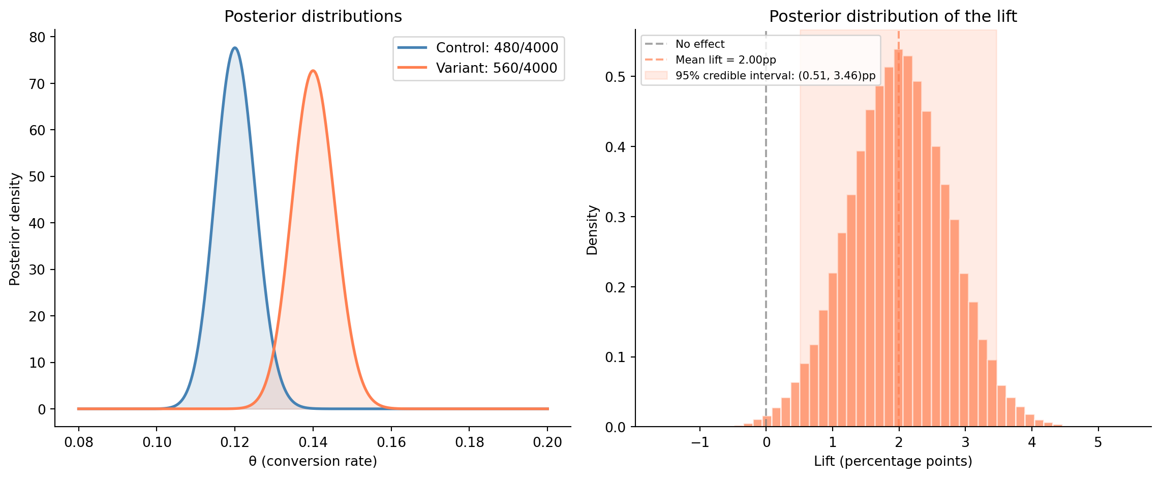
#| fig-cap: "Bayesian A/B test. Left: posterior distributions for each group's conversion rate. Right: posterior distribution of the lift (variant minus control), with the 95% credible interval shaded."
#| fig-alt: "Two-panel figure. First panel: two overlapping posterior density curves — control (solid blue, peaked near 0.12) and variant (dashed orange, peaked near 0.14) — with the variant shifted rightward toward higher conversion rates. Second panel: histogram of lift values in percentage points, centred near 2pp, with the 95% credible interval shaded in orange and a dotted grey line at zero indicating no effect."
fig, (ax1, ax2) = plt.subplots(1, 2, figsize=(12, 5))
fig.patch.set_alpha(0)
ax1.patch.set_alpha(0)
ax2.patch.set_alpha(0)

# Left: overlapping posteriors
theta = np.linspace(0.08, 0.20, 500)
ax1.plot(theta, posterior_control.pdf(theta), '#0072B2', linewidth=2,
         linestyle='-', label=f'Control: {conversions_control}/{n_control}')
ax1.plot(theta, posterior_variant.pdf(theta), '#E69F00', linewidth=2,
         linestyle='--', label=f'Variant: {conversions_variant}/{n_variant}')
ax1.fill_between(theta, posterior_control.pdf(theta), alpha=0.2, color='#0072B2')
ax1.fill_between(theta, posterior_variant.pdf(theta), alpha=0.2, color='#E69F00')
ax1.set_xlabel('θ (conversion rate)')
ax1.set_ylabel('Posterior density')
ax1.set_title("Variant's distribution sits to the right of control's", fontsize=10)
ax1.legend()
ax1.spines[['top', 'right']].set_visible(False)

# Right: lift distribution
# For Monte Carlo samples, we use np.percentile rather than ppf,
# since we're summarising draws, not evaluating a distribution object
ax2.hist(lift_samples * 100, bins=50, density=True, color='#E69F00',
         alpha=0.7)
ci_lo = np.percentile(lift_samples, 2.5) * 100
ci_hi = np.percentile(lift_samples, 97.5) * 100
ax2.axvline(0, color='grey', linestyle=':', alpha=0.7, label='No effect')
ax2.axvline(np.mean(lift_samples) * 100, color='#E69F00', linestyle='-',
            alpha=0.7, label=f'Mean lift = {np.mean(lift_samples)*100:.2f}pp')
ax2.axvspan(ci_lo, ci_hi, alpha=0.15, color='#E69F00',
            label=f'95% credible interval: ({ci_lo:.2f}, {ci_hi:.2f})pp')
ax2.set_xlabel('Lift (percentage points)')
ax2.set_ylabel('Density')
ax2.set_title('Posterior distribution of the lift', fontsize=10)
ax2.legend(fontsize=8)
ax2.spines[['top', 'right']].set_visible(False)

plt.tight_layout()
plt.show()
```
@fig-bayesian-ab shows the result. The Bayesian A/B test also handles the peeking problem from @sec-peeking differently. The posterior is a valid probability distribution at any sample size: you can examine it whenever you like without the posterior probability itself being distorted. By contrast, a frequentist p-value is valid at any single look, but using a fixed $\alpha$ threshold repeatedly as data accumulates inflates the false positive rate beyond $\alpha$ (as we saw in @sec-peeking). The posterior simply becomes more precise as data accumulates.
However, this does not mean you can peek freely and act on the result. Decision rules based on posterior thresholds (e.g., "ship when $P(\text{variant better}) > 0.95$") can still produce poorly calibrated conclusions with early stopping; the stated probabilities don't match how often the conclusions are actually correct.
The posterior itself is always a valid probability distribution, but *when* you choose to act on it affects your long-run error rate. With very small samples, the posterior is wide and dominated by the prior, so stopping early gives you an answer that reflects your assumptions more than your data. The answer is always valid — it just might not be very informative.
## From point estimates to distributions {#sec-posterior-predictive}
One of the most practically useful outputs of Bayesian inference is the **posterior predictive distribution**, the distribution of future observations, given the data you've seen.
Continuing with our A/B test variant ($560$ conversions in $4{,}000$ visitors), a frequentist would estimate $\hat{p} = 560/4{,}000 = 0.14$ (the hat denoting an estimate from data) and predict the next 1,000 visitors will produce $140$ conversions. This ignores the uncertainty in $\hat{p}$. The Bayesian approach integrates over all plausible values of $\theta$, weighting each prediction by the posterior probability of that $\theta$. In code, this is straightforward: draw a value of $\theta$ from the posterior, simulate data using that $\theta$, and repeat many times. The resulting spread accounts for both randomness in the data and uncertainty in the parameter.
```{python}
#| label: posterior-predictive
#| echo: true
# Predict conversions in the next 1,000 visitors (variant group),
# accounting for uncertainty in the conversion rate
n_future = 1000
point_estimate = conversions_variant / n_variant

# For each posterior sample of theta, simulate future conversions —
# each draw uses a different theta, which is the "integrate over theta" step
future_conversions = rng.binomial(n_future, samples_variant[:10_000])

print(f"Predicted conversions in next {n_future:,} visitors (variant):")
print(f"  Mean:   {np.mean(future_conversions):.0f}")
print(f"  Median: {np.median(future_conversions):.0f}")
print(f"  95% prediction interval: "
      f"({np.percentile(future_conversions, 2.5):.0f}, "
      f"{np.percentile(future_conversions, 97.5):.0f})")
print(f"\nPoint estimate prediction: {point_estimate * n_future:.0f}")
print(f"(ignores parameter uncertainty)")
```
The posterior predictive interval is wider than what you'd get from a point estimate alone, because it accounts for two sources of uncertainty: sampling variability (randomness in future outcomes even if you knew $\theta$ exactly) and parameter uncertainty (you don't know $\theta$ exactly). This is the same distinction we explored in @sec-standard-error, but now both sources are integrated naturally.
::: {.callout-note}
## Engineering Bridge
The posterior predictive distribution is analogous to **capacity planning under uncertainty**. When you provision at p99, you are not trusting the mean; you are asking where the parameter likely sits under realistic variability. The posterior predictive formalises this: it separates "my estimate of the rate is uncertain" (parameter uncertainty) from "even if I knew the rate exactly, individual outcomes would vary" (sampling variability), then combines both into a single prediction interval. The result is honest error bars that reflect everything you don't know.
:::
## When to go Bayesian {#sec-when-bayesian}
Bayesian inference isn't always the right choice, and choosing between Bayesian and frequentist methods is a practical decision, not an ideological one.
Bayesian inference earns its keep when you have genuine prior information worth incorporating: past experiments, domain constraints, or industry benchmarks that would be wasteful to ignore. It also works well when stakeholders want direct probability statements ("there's an 89% chance the variant is better" rather than "we reject $H_0$ at $\alpha = 0.05$"). Small samples are another sweet spot: the prior provides useful regularisation (pulling estimates away from extreme values) that a frequentist analysis cannot. And if you're running a continuous experiment, the posterior gives you valid inference at any stopping point.
Frequentist methods are the better choice when you need a well-established, widely accepted procedure; regulatory settings and academic publication still expect them. They're also the simpler choice when the sample is large enough that the prior is irrelevant and both approaches agree anyway, or when computational simplicity matters (a z-test is one line of code; a Bayesian model requires more setup). Frequentist guarantees on long-run error rates also hold regardless of the prior, which matters when you need to control false positive rates across many experiments.
In industry, the two approaches are increasingly used together. Many experimentation platforms run frequentist tests as the primary analysis (for their well-understood error guarantees) and offer Bayesian summaries as a complement (for their interpretability). You don't have to choose one camp — learn both, and apply whichever fits the problem.
## Worked example: monitoring alert calibration {#sec-bayesian-worked-example}
Let's return to the monitoring context from @sec-bayes. There, we assumed we knew the false positive rate and computed $P(\text{incident} \mid \text{alert})$. Now we flip the problem: we've observed alert outcomes and want to *estimate* the false positive rate itself, with uncertainty.
Your alerting system has been running for a month. You've received 200 alerts, and your team investigated each one. Of those 200, 18 were real incidents and 182 were false positives.
**Question:** What is the true false positive rate of your alerting system, and how uncertain should you be about it?
```{python}
#| label: alert-calibration
#| echo: true
# Data: 200 alerts, 182 false positives, 18 real incidents
n_alerts = 200
n_false_positives = 182
n_real = 18

# Prior: weakly informative, centred on 80% FP rate
# (reflecting industry experience that most alerts are noise)
alpha_prior, beta_prior = 8, 2  # Prior mean = 8/10 = 0.80

# Posterior for the false positive rate
alpha_post = alpha_prior + n_false_positives
beta_post = beta_prior + n_real

fp_posterior = stats.beta(alpha_post, beta_post)

print(f"Prior:     Beta({alpha_prior}, {beta_prior}) — "
      f"mean = {alpha_prior/(alpha_prior+beta_prior):.2f}")
print(f"Data:      {n_false_positives} FPs out of {n_alerts} alerts")
print(f"Posterior: Beta({alpha_post}, {beta_post})")
print(f"\nEstimated FP rate:  {fp_posterior.mean():.4f}")
print(f"95% credible interval: "
      f"({fp_posterior.ppf(0.025):.4f}, {fp_posterior.ppf(0.975):.4f})")
print(f"\nP(FP rate > 0.90) = {1 - fp_posterior.cdf(0.90):.4f}")
print(f"P(FP rate > 0.85) = {1 - fp_posterior.cdf(0.85):.4f}")
```
The posterior tells us the false positive rate is approximately 90% (95% credible interval: roughly 86% to 94%). The MLE is $182/200 = 91\%$, but the prior (centred at 80%) pulls the posterior mean slightly below that, a small but genuine demonstration that even a weak prior shifts the estimate. You can also read off actionable probabilities directly: there's a high probability the FP rate exceeds 85%, which might trigger a review of your alerting thresholds.
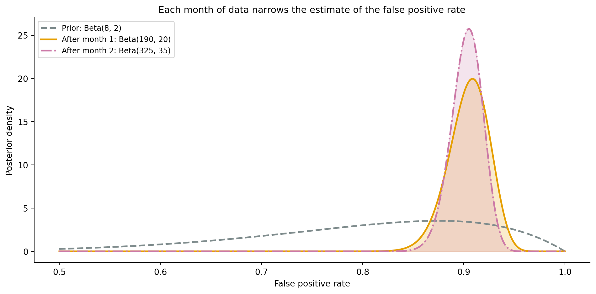
Now suppose you run the same alerting system for a second month without changing anything. This time, 150 alerts fire: 135 false positives and 15 real incidents. The beauty of Bayesian updating is that your current posterior becomes the prior for the next round; you don't start from scratch.
```{python}
#| label: fig-sequential-update
#| echo: true
#| fig-cap: "Sequential Bayesian updating. After the first month, the posterior (solid orange) reflects 200 alerts' worth of evidence. After a second month with 150 more alerts, the posterior (dash-dot purple) is narrower — more data means less uncertainty."
#| fig-alt: "Line chart showing three distributions over false positive rate from 0.5 to 1.0. The initial prior (dashed, labelled 'Prior: Beta(8, 2)') is broad and peaked near 0.80. The 'After month 1' posterior (solid amber) is taller and narrower, peaked near 0.91. The 'After month 2' posterior (dash-dot purple) is taller still and narrower, demonstrating that each additional month of data reduces uncertainty about the false positive rate."
# Second round of data (same system, second month)
n_alerts_2 = 150
n_fp_2 = 135
n_real_2 = 15

# The posterior from round 1 becomes the prior for round 2
alpha_post_2 = alpha_post + n_fp_2
beta_post_2 = beta_post + n_real_2

fp_posterior_2 = stats.beta(alpha_post_2, beta_post_2)

fig, ax = plt.subplots(figsize=(10, 5))
fig.patch.set_alpha(0)
ax.patch.set_alpha(0)
theta = np.linspace(0.5, 1.0, 500)

# Prior
prior_dist = stats.beta(alpha_prior, beta_prior)
ax.plot(theta, prior_dist.pdf(theta), '#7f8c8d', linewidth=2,
        linestyle='--', label=f'Prior: Beta({alpha_prior}, {beta_prior})')

# After month 1
ax.plot(theta, fp_posterior.pdf(theta), '#E69F00', linewidth=2,
        linestyle='-', label=f'After month 1: Beta({alpha_post}, {beta_post})')
ax.fill_between(theta, fp_posterior.pdf(theta), alpha=0.2, color='#E69F00')

# After month 2
ax.plot(theta, fp_posterior_2.pdf(theta), '#CC79A7', linewidth=2,
        linestyle='-.', label=f'After month 2: Beta({alpha_post_2}, {beta_post_2})')
ax.fill_between(theta, fp_posterior_2.pdf(theta), alpha=0.2, color='#CC79A7')

ax.set_xlabel('False positive rate')
ax.set_ylabel('Posterior density')
ax.set_title('Each month of data narrows the estimate of the false positive rate',
             fontsize=11)
ax.legend(fontsize=9)
ax.spines[['top', 'right']].set_visible(False)
plt.tight_layout()
plt.show()

print(f"After month 2:")
print(f"  Estimated FP rate: {fp_posterior_2.mean():.4f}")
print(f"  95% credible interval: "
      f"({fp_posterior_2.ppf(0.025):.4f}, {fp_posterior_2.ppf(0.975):.4f})")
print(f"  P(FP rate > 0.90) = {1 - fp_posterior_2.cdf(0.90):.4f}")
```
@fig-sequential-update shows the result. The posterior is narrower after the second month (more data means less uncertainty) and the sequential updating naturally incorporated all the evidence from both months. This is the key advantage: Bayesian updating is inherently incremental. Each batch of data refines your estimate without discarding what came before. Note that this works because the underlying system didn't change between months. If you had tuned the alerting thresholds between months, you'd be estimating a *different* parameter and would need a fresh prior for the new regime.
## Summary {#sec-bayesian-inference-summary}
1. **Bayesian inference treats parameters as uncertain quantities** with probability distributions, not fixed unknowns. The posterior distribution captures everything you know about a parameter after seeing the data.
2. **Posterior $\propto$ likelihood $\times$ prior.** The prior encodes what you knew before; the likelihood encodes what the data says; the posterior combines them. With enough data, the prior becomes irrelevant.
3. **Credible intervals mean what you think they mean.** A 95% credible interval contains the parameter with 95% probability — no hypothetical repetitions required.
4. **Bayesian A/B testing gives direct probability statements** — "there's a greater than 99% chance the variant is better" — rather than the frequentist "we reject $H_0$ at $\alpha = 0.05$."
5. **Bayesian updating is sequential by nature.** Each posterior becomes the next prior, making it natural for ongoing experiments, monitoring, and iterative learning.
## Exercises {#sec-bayesian-inference-exercises}
1. A new feature has a bug rate you want to estimate. In the first week, you observe 3 bugs across 500 user sessions. Compute the posterior distribution using a Beta$(1, 1)$ prior. What is the 95% credible interval for the bug rate? Now suppose a colleague tells you that similar features historically have a bug rate around 1%. Repeat the analysis with a Beta$(2, 198)$ prior (centred at 1%). How does the credible interval change, and why?
2. **Simulate the prior's influence.** Using a true conversion rate of $p = 0.15$, generate data at four sample sizes: $n \in \{10, 50, 200, 500\}$ Bernoulli trials. For each sample size, compute the posterior under three priors: Beta$(1, 1)$, Beta$(5, 45)$, and Beta$(50, 450)$. Plot all three posteriors for each sample size. At what sample size do the posteriors converge regardless of the prior?
3. Repeat the Bayesian A/B test from @sec-bayesian-ab, but with smaller samples: 40 visitors per group, with 5 conversions (control) and 8 conversions (variant). Compute $P(\text{variant} > \text{control})$. Now try the frequentist test (`scipy.stats.fisher_exact` — an exact test for 2×2 contingency tables that works well with small samples, unlike the large-sample z-test from @sec-two-sample-test). Which approach gives you a more useful answer with this little data, and why?
4. **Sequential updating exercise.** Simulate a stream of Bernoulli observations with $p = 0.30$. Start with a Beta$(1, 1)$ prior. After each observation, update the posterior and record the 95% credible interval. Plot the credible interval width as a function of the number of observations. How many observations does it take for the interval width to drop below 0.10?
5. **Conceptual:** A frequentist and a Bayesian analyse the same A/B test data. The frequentist reports $p = 0.048$ (just significant at $\alpha = 0.05$). The Bayesian, using a sceptical prior (one that places most of its weight on small or zero effects), reports $P(\text{variant better}) = 0.82$. Neither is wrong. Explain how they can reach different conclusions from the same data, and in what business context each answer would be more useful.