---
# Content: CC BY-NC-SA 4.0 | Code: MIT - see /LICENSE.md
title: "A/B testing: deploying experiments"
---
{{< include /_common-imports.qmd >}}
## From feature flags to controlled experiments {#sec-ab-testing}
You already run experiments in production. Every canary deployment is one: route a fraction of traffic to the new version, watch the dashboards, roll back if something breaks. Feature flags let you enable functionality for a subset of users and measure the impact before a full rollout.
A/B testing formalises this instinct. Instead of eyeballing dashboards and hoping you'd notice a problem, you define the question upfront, decide how much data you need, and randomly split your users. Then you apply the statistical machinery from the previous two chapters to determine whether the difference is real. The ingredients — hypothesis testing (@sec-testing-framework), confidence intervals (@sec-confidence-intervals), and power analysis (@sec-power) — are all in place. This chapter is about assembling them into a reliable experimental process.
The payoff is substantial. Without a formal experiment, you're left with "the conversion rate went up after we shipped the new checkout flow", but you don't know whether that's the new flow, a seasonal trend, a marketing campaign, or noise. With a randomised experiment, you can attribute the difference to the change you made, because the only systematic difference between the two groups is the intervention.
## Designing the experiment {#sec-experiment-design}
Before writing any code, an A/B test requires four design decisions. Each one constrains the next, so they form a chain: the metric you choose determines what counts as a meaningful effect, the minimum detectable effect drives the sample size, and the sample size together with your traffic determines the runtime.
The first decision is the **unit of randomisation**, usually individual users, but sometimes sessions, devices, or geographic regions. The unit must be stable: if a user refreshes the page and lands in the other group, you've contaminated your experiment. Hash-based assignment solves this by hashing the user ID to deterministically assign them to a group.
```{python}
#| label: hash-assignment
#| echo: true
import hashlib

def assign_group(user_id: str, experiment: str, n_groups: int = 2) -> int:
    """Deterministic group assignment via hashing.

    Same user + same experiment = same group, every time.
    Different experiments get independent assignments.
    """
    # Include experiment name so a user's assignment in one test
    # is independent of their assignment in another.
    key = f"{experiment}:{user_id}".encode()
    hash_val = int(hashlib.sha256(key).hexdigest(), 16)
    return hash_val % n_groups

# Demonstrate stability and uniformity
users = [f"user_{i}" for i in range(10_000)]
groups = [assign_group(uid, 'checkout_redesign_2024') for uid in users]
counts = np.bincount(groups)
print(f"Group 0 (control): {counts[0]:,}")
print(f"Group 1 (variant): {counts[1]:,}")
print(f"Ratio: {counts[0]/counts[1]:.3f}  (ideal: 1.000)")
```
This approach has three properties you want: it's deterministic (no state to manage), approximately uniform (the split is balanced for large samples, though any finite sample will show small deviations), and independent across experiments (a user's assignment in one test doesn't affect another). Always verify the actual split empirically; we'll see how to detect a problem in the section on sample ratio mismatch below.
Next, choose the **primary metric**, the one your decision hinges on, whether that is conversion rate, revenue per user, latency, or error rate. Fix it before the experiment starts. You will also want **guardrail metrics**: things that should not get worse even if the primary metric improves. A checkout redesign might increase conversion but also increase page load time or support tickets.
The primary metric feeds into the third decision: the **minimum detectable effect** (MDE), the smallest change worth detecting. If a 0.5 percentage point conversion lift is not worth the engineering cost of maintaining the new checkout flow, do not design the test to detect it; you would need an impractically large sample. Be honest about this: what is the smallest improvement that would change your decision?
Finally, decide the **runtime**, long enough to reach the required sample size from your power analysis. Not longer, and critically, not shorter; we will see why in @sec-peeking.
::: {.callout-note}
## Engineering Bridge
This design phase is the **requirements specification** of an experiment. Just as you wouldn't start coding without knowing the acceptance criteria, you shouldn't start an A/B test without specifying the metric, the minimum detectable effect, the sample size, and the decision rule. Changing any of these after seeing the data is the statistical equivalent of modifying your test assertions to match the output; it invalidates the result.
:::
## Planning the sample size {#sec-sample-size-planning}
In @sec-power, we computed the sample size needed to detect a specific effect. Now let's apply that to a realistic planning scenario.
Your checkout currently converts at 12%. The product team believes the redesign will improve this by at least 2 percentage points (pp); anything less wouldn't justify the cost. You want 80% power at $\alpha = 0.05$ (the significance level, the false positive rate you're willing to tolerate, from @sec-testing-framework). To calculate the required sample size, we first convert the 2pp difference into a standardised effect size using Cohen's h, which we introduced in @sec-power. The arcsine transformation at the heart of Cohen's h accounts for the fact that proportions near 0% or 100% are inherently less variable than those near 50%.
```{python}
#| label: sample-size-planning
#| echo: true
from statsmodels.stats.power import NormalIndPower

# Power analysis for two independent groups using the Normal approximation —
# suitable for comparing proportions at reasonable sample sizes (see @sec-power).
power_analysis = NormalIndPower()

baseline = 0.12
minimum_detectable_effect = 0.02  # 2 percentage points
target = baseline + minimum_detectable_effect

# Cohen's h: standardised effect size for proportions.
# The arcsine-sqrt transformation puts proportion differences on a common scale.
cohens_h = 2 * (np.arcsin(np.sqrt(target)) - np.arcsin(np.sqrt(baseline)))

n_per_group = power_analysis.solve_power(
    effect_size=cohens_h,
    alpha=0.05,
    power=0.80,
    alternative='two-sided'
)

n_per_group = int(np.ceil(n_per_group))

print(f"Baseline rate:     {baseline:.0%}")
print(f"Target rate:       {target:.0%}")
print(f"MDE:               {minimum_detectable_effect * 100:.1f}pp")
print(f"Cohen's h:         {cohens_h:.4f}")
print(f"Required n/group:  {n_per_group:,}")
print(f"Total users:       {2 * n_per_group:,}")
```
Cohen's h is the standard effect-size measure for comparing two proportions:
$$h = 2\left(\arcsin\sqrt{p_1} - \arcsin\sqrt{p_0}\right)$$
The arcsine transformation stabilises variance across different baseline rates, so the same $h$ represents a comparable "difficulty of detection" whether your baseline is 5% or 50%.
Now translate that into a runtime estimate. If your site gets 5,000 checkout-eligible users per day and you split them 50/50:
```{python}
#| label: runtime-estimate
#| echo: true
daily_traffic = 5000
users_per_group_per_day = daily_traffic / 2

days_needed = int(np.ceil(n_per_group / users_per_group_per_day))

print(f"Daily eligible users: {daily_traffic:,}")
print(f"Per group per day:    {users_per_group_per_day:,.0f}")
print(f"Days to reach n:      {days_needed}")
print(f"\nPlan for {days_needed} days — round up to "
      f"{int(np.ceil(days_needed / 7)) * 7} days to capture full weekly cycles.")
```
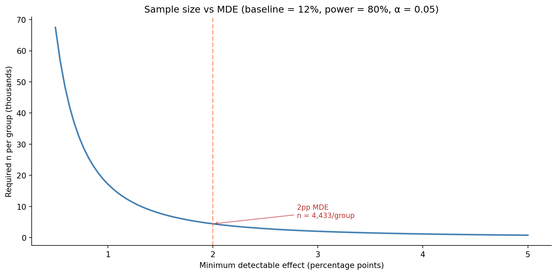
Running for complete weeks matters. User behaviour varies by day of week (weekend shoppers behave differently from weekday browsers), and cutting an experiment mid-week introduces a subtle bias. Always round up to a whole number of weeks. @fig-sample-size-tradeoffs shows how the required sample size changes as you vary the MDE.
```{python}
#| label: fig-sample-size-tradeoffs
#| echo: true
#| fig-cap: "The relationship between minimum detectable effect and required sample size. Smaller effects demand dramatically more data — a 1 pp (percentage point) MDE requires roughly four times the sample of a 2 pp MDE."
#| fig-alt: "Line chart showing required sample size per group (y-axis, thousands) against minimum detectable effect in percentage points (x-axis). The curve falls steeply from left to right: at 0.5pp the required n exceeds 67,000 per group, while at 2pp it drops to around 4,400. A dashed annotation marks the 2pp MDE used in this chapter's worked example."
mde_range = np.linspace(0.005, 0.05, 100)
n_required = []

# solve_power requires scalar inputs, so we loop rather than vectorise
for mde in mde_range:
    h = 2 * (np.arcsin(np.sqrt(baseline + mde)) - np.arcsin(np.sqrt(baseline)))
    n = power_analysis.solve_power(
        effect_size=h, alpha=0.05, power=0.80, alternative='two-sided'
    )
    n_required.append(n)

fig, ax = plt.subplots(figsize=(10, 5))
fig.patch.set_alpha(0)
ax.patch.set_alpha(0)
ax.plot(mde_range * 100, np.array(n_required) / 1000, '#0072B2', linewidth=2)
ax.set_xlabel('Minimum detectable effect (percentage points)')
ax.set_ylabel('Required n per group (thousands)')
ax.set_title('Detecting smaller effects demands far more data\n'
             '(sample size grows as roughly 1/MDE²; baseline = 12%, power = 80%, α = 0.05)',
             fontsize=11)

# Mark the 2pp MDE
ax.axvline(2.0, color='#333', linestyle='--', alpha=0.9)
ax.annotate(f'2pp MDE\nn = {n_per_group:,}/group',
            xy=(2.0, n_per_group / 1000), xytext=(2.8, n_per_group / 1000 + 2),
            fontsize=9, color='#333',
            arrowprops=dict(arrowstyle='->', color='#333', alpha=0.9))

ax.spines[['top', 'right']].set_visible(False)
plt.tight_layout()
plt.show()
```
::: {.callout-tip}
## Author's Note
The most dangerous outcome of an A/B test is an *uninformative* answer that gets treated as a real one. When a test is underpowered (too small a sample), failing to reject $H_0$ tells you nothing, but stakeholders will read it as "the feature doesn't work." That conflation between "we didn't detect a difference" and "there is no difference" is remarkably hard to correct after the fact. Running the power analysis first and committing to the required timeline *before* the experiment starts is the only reliable defence. It feels like overhead; it's actually the most important step.
:::
## Guardrail metrics and multiple testing {#sec-guardrail-metrics}
A single primary metric isn't enough. You need to monitor secondary metrics, **guardrails**, that should not degrade. A new checkout flow that improves conversion by 2pp but increases page load time by 500ms or doubles the support ticket rate is not a win.
The problem is that every additional metric you test increases your chance of a false positive. Test 10 guardrails at $\alpha = 0.05$ each, and you have roughly a 40% chance of at least one false alarm, even when nothing is wrong. (This calculation assumes independent tests. Positively correlated metrics, common in practice, give a lower true FWER, so the formula is a conservative upper bound.)
```{python}
#| label: multiple-testing-risk
#| echo: true
n_metrics = np.arange(1, 21)
p_any_false_positive = 1 - (1 - 0.05) ** n_metrics

print(f"{'Metrics tested':>15}  {'P(≥1 false positive)':>22}")
print('-' * 40)
for n, p in zip(n_metrics[::2], p_any_false_positive[::2]):
    print(f"{n:>15}  {p:>22.1%}")
```
The **Bonferroni correction** (a multiple-testing adjustment we flagged in @sec-p-value-pitfalls) is the simplest fix: divide $\alpha$ by the number of guardrails. With 10 guardrails, use $\alpha = 0.005$ for each. This controls the **family-wise error rate** (FWER), the probability of *at least one* false positive across all the tests you run, but it's conservative. If you have 20 metrics, Bonferroni demands $p < 0.0025$, which reduces your power to detect real problems.
In practice, A/B testing platforms often distinguish between the **primary metric** (tested at the full $\alpha$) and **guardrails** (tested at a corrected $\alpha$ or monitored without formal testing). The primary metric drives the launch decision; guardrails catch unexpected harm. Note that this approach does not control the overall FWER across *all* tests (primary + guardrails) to 0.05; only the guardrails are corrected. The rationale is that the primary metric and guardrails serve different roles, so controlling them separately is more appropriate than a single correction across everything.
```{python}
#| label: bonferroni-guardrails
#| echo: true
from scipy import stats

alpha = 0.05
n_guardrails = 5

# Primary metric tested at full alpha; correct guardrails only
alpha_corrected = alpha / n_guardrails

print(f"Primary metric threshold:  α = {alpha:.3f}")
print(f"Number of guardrails:      {n_guardrails}")
print(f"Guardrail threshold:       α = {alpha_corrected:.4f}")
print(f"Guardrail FWER:            ≤ {alpha:.3f}")
print(f"  (covers guardrails only — the primary adds its own α)")

# What z-score does this correspond to?
z_corrected = stats.norm.ppf(1 - alpha_corrected / 2)  # inverse CDF: z for a given tail area
print(f"\nCritical z (guardrail):    {z_corrected:.3f}")
print(f"Critical z (primary):      {stats.norm.ppf(0.975):.3f}")
```
## The peeking problem {#sec-peeking}
The most common mistake in A/B testing isn't choosing the wrong test or the wrong metric — it's looking at the results too early and stopping when you see significance.
This seems harmless. Why not check the dashboard daily and stop as soon as the result is clear? Because the p-value (the probability of seeing data this extreme if there is no real effect) is only valid for a single, *pre-committed* analysis. If you check every day and stop the first time $p < 0.05$, you're running a different experiment, one with a much higher false positive rate.
The simulation below uses the two-proportion z-test at each daily check. Writing $\hat{p}_c$ and $\hat{p}_v$ for the observed conversion rates in the control and variant groups, $n_c$ and $n_v$ for the respective group sizes, and $\hat{p}$ for the pooled proportion across both groups, the test statistic is:
$$z = \frac{\hat{p}_v - \hat{p}_c}{\sqrt{\hat{p}(1-\hat{p})\left(\frac{1}{n_c} + \frac{1}{n_v}\right)}}$$
Under $H_0$ (no difference), $z$ follows a standard Normal distribution; this is the same standardisation logic from @sec-testing-framework, now applied to the difference in proportions rather than a single mean.
```{python}
#| label: fig-peeking-simulation
#| echo: true
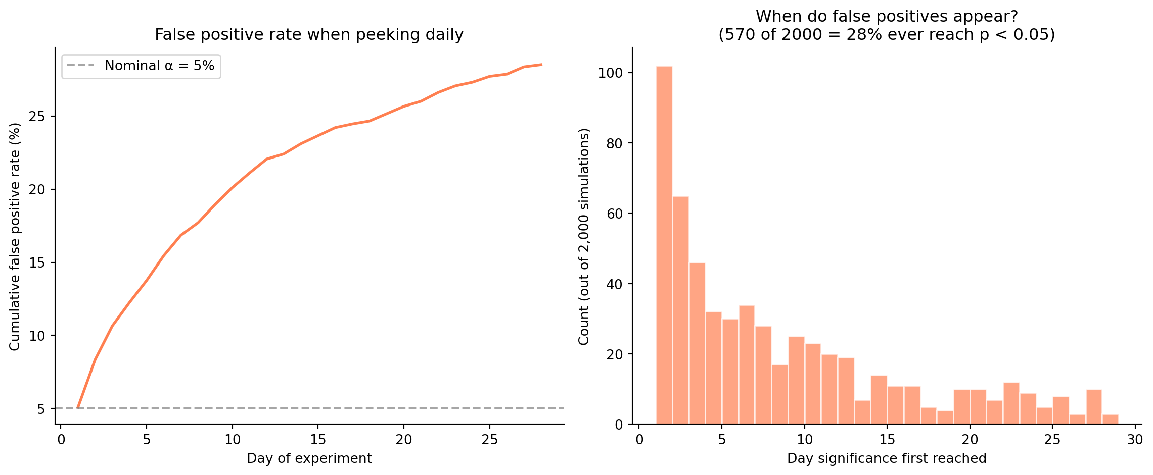
#| fig-cap: "Peeking inflates false positives. The cumulative false positive rate rises well above the nominal 5% as daily checks accumulate over 28 days. The day-of-first-significance histogram shows that most spurious results appear in the opening days, when sample sizes are small and estimates are noisy."
#| fig-alt: "Two-panel figure. Left panel: line chart of cumulative false positive rate (y-axis, percent) over experiment days (x-axis). The rate climbs from near 0% on day 1 to roughly 25–30% by day 28, far exceeding the dashed 5% nominal alpha line. Right panel: histogram of the day each false positive first reaches significance, showing a concentration of spurious results in the first week."
rng = np.random.default_rng(42)

true_rate = 0.10  # Same rate for both groups — no real effect
n_per_day = 500   # Users per group per day
max_days = 28
n_simulations = 2000

# Track when each simulation first reaches significance
first_sig_day = []
ever_significant = 0

for _ in range(n_simulations):
    control_total = 0
    variant_total = 0
    control_conversions = 0
    variant_conversions = 0
    found_sig = False

    for day in range(1, max_days + 1):
        # New data each day
        control_conversions += rng.binomial(n_per_day, true_rate)
        variant_conversions += rng.binomial(n_per_day, true_rate)
        control_total += n_per_day
        variant_total += n_per_day

        # Test at current accumulated data
        p_c = control_conversions / control_total
        p_v = variant_conversions / variant_total
        p_pooled = (control_conversions + variant_conversions) / (control_total + variant_total)
        se = np.sqrt(p_pooled * (1 - p_pooled) * (1/control_total + 1/variant_total))

        if se > 0:
            # z-test for two proportions (see hypothesis testing chapter)
            z = (p_v - p_c) / se
            # sf = survival function = P(Z > z), i.e. 1 - CDF; ×2 for two-sided
            p_val = 2 * stats.norm.sf(abs(z))

            if p_val < 0.05 and not found_sig:
                first_sig_day.append(day)
                found_sig = True

    if found_sig:
        ever_significant += 1

fig, (ax1, ax2) = plt.subplots(1, 2, figsize=(12, 5))
fig.patch.set_alpha(0)
ax1.patch.set_alpha(0)
ax2.patch.set_alpha(0)

# Left: cumulative false positive rate over time
fp_by_day = [sum(1 for d in first_sig_day if d <= day) / n_simulations
             for day in range(1, max_days + 1)]

ax1.plot(range(1, max_days + 1), [f * 100 for f in fp_by_day],
         '#E69F00', linewidth=2, label='Actual false positive rate (peeking)')
ax1.axhline(5, color='grey', linestyle='--', alpha=0.7)
ax1.annotate('Nominal α = 5%', xy=(1, 5), xytext=(1, 6.5),
             fontsize=9, color='grey', va='bottom')
ax1.set_xlabel('Day of experiment')
ax1.set_ylabel('Cumulative false positive rate (%)')
ax1.set_title('Daily peeking inflates false positives to ~25–30%', fontsize=10)
ax1.spines[['top', 'right']].set_visible(False)

# Right: histogram of when false positives occur
ax2.hist(first_sig_day, bins=range(1, max_days + 2), color='#E69F00',
         edgecolor='#ccc', alpha=0.85)
ax2.set_xlabel('Day significance first reached')
ax2.set_ylabel('Count (out of 2,000 simulations)')
ax2.set_title(f'Most false positives appear early\n'
              f'({ever_significant} of {n_simulations} = '
              f'{ever_significant/n_simulations:.0%} ever reach p < 0.05)',
              fontsize=10)
ax2.spines[['top', 'right']].set_visible(False)

plt.tight_layout()
plt.show()
```
@fig-peeking-simulation shows that with daily peeking and no correction, the false positive rate inflates well beyond 5%, typically reaching 25–30% over a four-week experiment. Many of the false alarms occur early, when the sample is small and the estimates are noisy.
There are three practical solutions:
1. **Don't peek.** Decide the runtime upfront, run the full duration, and analyse once. This is the simplest approach and works well when you can commit to the timeline.
2. **Use sequential testing.** Methods like the **O'Brien–Fleming** group sequential design allow you to check at pre-specified interim points, for instance at 25%, 50%, and 75% of the planned sample, with adjusted significance thresholds that maintain the overall $\alpha$. Early checks use very stringent thresholds (for example, $p < 0.001$ at the 25% interim, relaxing toward $p \approx 0.05$ at the final analysis), making it hard to stop early on noise.
3. **Use always-valid inference.** More recent approaches provide inference that's valid at any stopping time: you can check continuously without inflating the error rate. **Confidence sequences** are intervals that remain valid no matter when you check them (unlike the fixed-sample CIs from @sec-confidence-intervals), and **e-values** measure evidence that can be accumulated over time without adjustment. The price of this flexibility is wider intervals at any given sample size compared to a fixed-sample analysis — you trade statistical efficiency for the freedom to stop whenever you choose. Modern experimentation platforms increasingly use these methods.
::: {.callout-note}
## Engineering Bridge
Peeking is the statistical equivalent of **repeatedly running your test suite on a feature branch and declaring "tests pass" the first time you get a green run**, even if previous runs failed. You're exploiting multiple attempts to get the answer you want. With flaky tests, each run has a small chance of a false green; re-run enough times and you'll get one. With A/B testing, each daily check has a small chance of a false positive; check enough times and you'll find one. The fix is the same in both cases: either run once at a pre-committed point, or use a procedure designed for repeated checking.
:::
## Interpreting results {#sec-interpreting-results}
The experiment has run its course. You have a p-value and a confidence interval. Now what?
The most useful output isn't the p-value — it's the CI for the difference, which we built in @sec-ci-proportion. The CI tells you three things at once: whether the effect is statistically significant (does it exclude zero?), how large the effect plausibly is (the range), and how precise your estimate is (the width).
```{python}
#| label: interpret-results
#| echo: true
# Illustrative figures, hand-chosen to give a clean ~2pp lift for this
# walkthrough — distinct from the simulated worked example later in the chapter.
n_control, n_variant = 4000, 4000
conversions_control = 480   # 12.0%
conversions_variant = 560   # 14.0%

p_c = conversions_control / n_control
p_v = conversions_variant / n_variant
diff = p_v - p_c

# CI uses unpooled SE — each group keeps its own variance estimate,
# because we're estimating the actual difference (not assuming H0: equal rates).
se_c = np.sqrt(p_c * (1 - p_c) / n_control)
se_v = np.sqrt(p_v * (1 - p_v) / n_variant)
se_diff = np.sqrt(se_c**2 + se_v**2)
# ppf = percent point function (inverse CDF): the z-value for a given tail area
z_crit = stats.norm.ppf(0.975)

ci_lower = diff - z_crit * se_diff
ci_upper = diff + z_crit * se_diff

# Hypothesis test uses pooled SE — under H0, both groups share the same rate.
p_pooled = (conversions_control + conversions_variant) / (n_control + n_variant)
se_pooled = np.sqrt(p_pooled * (1 - p_pooled) * (1/n_control + 1/n_variant))
z_stat = diff / se_pooled
p_value = 2 * stats.norm.sf(abs(z_stat))

print(f"Control:    {p_c:.1%} ({conversions_control}/{n_control})")
print(f"Variant:    {p_v:.1%} ({conversions_variant}/{n_variant})")
print(f"Difference: {diff:.1%}")
print(f"95% CI:     ({ci_lower:.1%}, {ci_upper:.1%})")
print(f"p-value:    {p_value:.4f}")
print(f"\nStatistically significant? {p_value < 0.05}")
print(f"CI excludes zero?          {ci_lower > 0 or ci_upper < 0}")
```
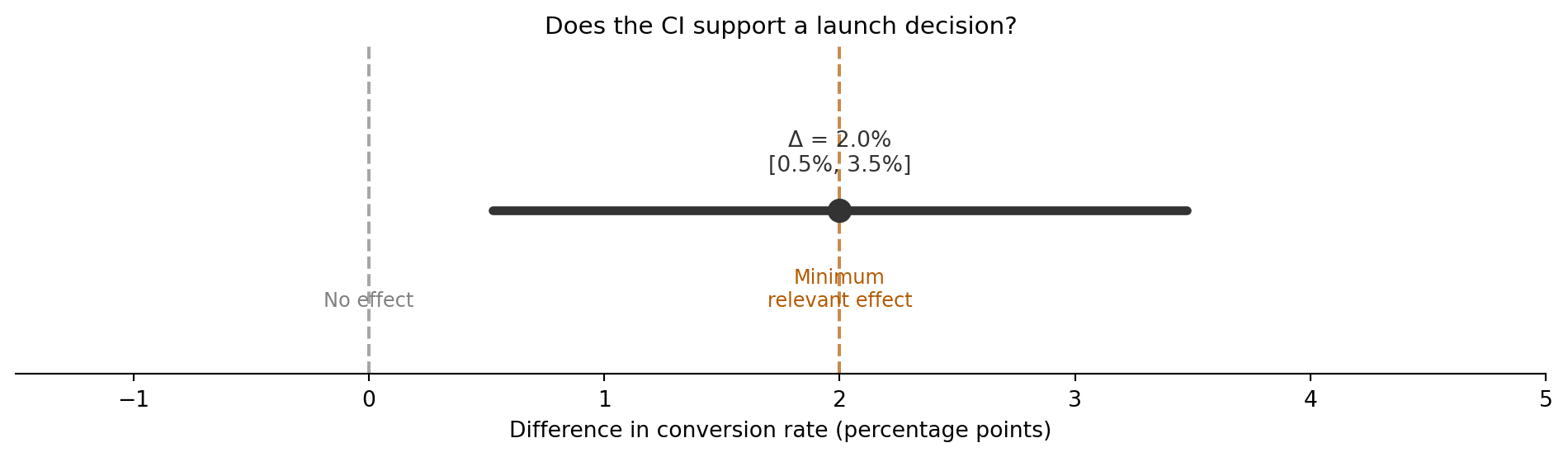
The CI tells us the true lift is plausibly between about 0.5 and 3.5 percentage points. That's a useful range for a decision. If even a 0.5 percentage point lift justifies shipping (because the feature has no ongoing cost), ship it. If you need at least 2 percentage points to justify the maintenance burden, the data is encouraging but not conclusive; the true effect could be below your threshold.
```{python}
#| label: fig-decision-framework
#| echo: true
#| fig-cap: "CI-based decision framework. The CI for the conversion rate difference is shown against two decision boundaries: zero (no effect) and the 2pp MDE. The entire CI sits above zero (significant), but it straddles the practical significance boundary."
#| fig-alt: "Horizontal confidence interval plot. A thick line segment representing the 95% CI for the conversion rate difference spans roughly 0.5 to 3.5 percentage points, with a point estimate around 2.0. Two vertical dashed lines mark boundaries: 'No effect' at zero and 'Minimum relevant effect' at 2 percentage points. The CI clears zero entirely but overlaps the MDE threshold."
fig, ax = plt.subplots(figsize=(10, 4))
fig.patch.set_alpha(0)
ax.patch.set_alpha(0)

# CI bar
ax.plot([ci_lower * 100, ci_upper * 100], [0, 0], color='#333',
        linewidth=4, solid_capstyle='round')
ax.plot(diff * 100, 0, 'o', color='#333', markersize=10, zorder=5)
ax.annotate(f'Δ = {diff:.1%}\n[{ci_lower:.1%}, {ci_upper:.1%}]',
            xy=(diff * 100, 0), xytext=(0, 18), textcoords='offset points',
            ha='center', fontsize=10, color='#333')

# Decision boundaries
for threshold, label, colour in [
    (0, 'No effect', '#555'),
    (2.0, 'Minimum\nrelevant effect', '#b35900'),
]:
    ax.axvline(threshold, color=colour, linestyle='--', alpha=0.8)
    ax.annotate(label, xy=(threshold, 0), xytext=(threshold, -0.4),
                ha='center', fontsize=9, color=colour)

ax.set_xlim(-1.5, 5.0)
ax.set_ylim(-0.8, 0.8)
ax.set_xlabel('Difference in conversion rate (percentage points)')
ax.set_yticks([])
ax.spines[['top', 'right', 'left', 'bottom']].set_visible(False)
ax.set_title('CI spans the MDE threshold — effect is real but magnitude is uncertain',
             fontsize=11)
plt.tight_layout()
plt.show()
```
The CI-based framework in @fig-decision-framework is more informative than a binary significant/not-significant call. It naturally incorporates both statistical and practical significance: you can see at a glance whether the plausible range of effects overlaps with your decision threshold.
## Common pitfalls {#sec-ab-pitfalls}
A/B tests fail in predictable ways. Most failures come not from the statistics but from the experimental design.
The first failure mode is interference between groups. If control and variant users interact — sharing a chat feature, competing for the same limited-time deals, affecting each other's recommendations — the independence assumption breaks down. The technical term is **spillover** (the treatment "leaks" from one group to the other), also called **network interference** when the leakage happens through social connections. The fix depends on the context: cluster randomisation (randomise entire units, such as teams, organisations, or geographic regions, rather than individual users, so that interactions stay within a group), geographic splitting, or time-based alternation.
A second common issue is **sample ratio mismatch** (SRM). If your 50/50 split consistently shows 51/49 or worse, something is biasing the assignment. Common causes include bots or crawlers that only trigger one variant, assignment logic that depends on something correlated with the outcome (like user age), or redirect-based implementations where one variant's page loads faster and captures more sessions. Always check the actual split before interpreting results.
```{python}
#| label: srm-check
#| echo: true
# Check whether a 50/50 split is actually balanced
observed_control = 4847
observed_variant = 5153
total = observed_control + observed_variant

# Chi-squared goodness-of-fit: tests whether observed counts match expected
# frequencies. With two groups and no explicit expected counts, scipy assumes
# equal allocation (50/50).
chi2, p_value = stats.chisquare([observed_control, observed_variant])

print(f"Control: {observed_control:,}  ({observed_control/total:.1%})")
print(f"Variant: {observed_variant:,}  ({observed_variant/total:.1%})")
print(f"χ² = {chi2:.2f}, p = {p_value:.4f}")

# Stricter threshold (0.01) than the usual 0.05 because a detected SRM
# invalidates the entire experiment — the cost of missing one is high.
if p_value < 0.01:
    print('WARNING: Sample ratio mismatch detected — investigate before interpreting results.')
else:
    print('Split looks balanced — no SRM concern.')
```
Then there is **Simpson's paradox**: an effect that appears in aggregate data can reverse when you look at subgroups, or vice versa. This happens when subgroups have different sizes or different baseline rates and the aggregation hides the imbalance. A checkout redesign might improve conversion overall, but only because it shifted the mix of mobile versus desktop users. Always check whether the effect is consistent across major segments (device type, new versus returning users, geography) before attributing it to the treatment.
Finally, watch for **novelty and primacy effects**. Users may react to a new design simply because it is new (novelty effect) or resist it because they are accustomed to the old design (primacy effect). Both fade with time. Running the experiment for at least two full weeks helps, and comparing early versus late behaviour can flag whether the effect is stable.
::: {.callout-tip}
## Author's Note
A green A/B test feels conclusive in the same way that a green CI build feels conclusive: the gates passed, you can ship. But a passing test only guarantees the *aggregate* effect was positive at this experiment's level of precision. That can hide a lot. The new checkout might lift conversion by 2 percentage points overall while quietly suppressing conversion for users on flaky mobile networks, or for first-time visitors, or for one specific browser. Aggregation averages those losses out. Engineers test for this kind of asymmetry all the time, just under different names, e.g., segmented monitoring after a release, or canary alerts that fire on a single region. The discipline carries straight over to experiments: a single significant lift at the top is the start of the analysis, not the end of it. Always inspect the major segments before declaring victory, and treat any subgroup that moves in the opposite direction as a finding worth understanding before launch.
:::
## Worked example: end-to-end experiment {#sec-ab-worked-example}
**The scenario.** Your e-commerce checkout currently converts at 12%. The product team has redesigned the payment step to reduce friction. You need to decide whether to launch the new design.
**Step 1: Design.** Primary metric: checkout conversion rate. Guardrails: page load time, payment error rate, average order value. MDE: 2 percentage points (the team agrees anything less isn't worth the migration). Significance: $\alpha = 0.05$. Power: 80%.
**Step 2: Sample size.** From our earlier calculation, we need approximately 4,400 users per group, roughly 8,800 total. At 5,000 eligible users per day (50/50 split), that's 2 days to reach the target, which we round up to 7 for a full weekly cycle.
**Step 3: Run and wait.** After 7 days, we have our data.
```{python}
#| label: full-experiment
#| echo: true
# Simulated experiment results after a full week
rng = np.random.default_rng(42)

# Simulate: true control rate 12%, true variant rate 14%
control_conversions = rng.binomial(n_per_group, 0.12)
variant_conversions = rng.binomial(n_per_group, 0.14)

p_c = control_conversions / n_per_group
p_v = variant_conversions / n_per_group
diff = p_v - p_c

# Primary metric: CI for the difference
se_c = np.sqrt(p_c * (1 - p_c) / n_per_group)
se_v = np.sqrt(p_v * (1 - p_v) / n_per_group)
se_diff = np.sqrt(se_c**2 + se_v**2)
z_crit = stats.norm.ppf(0.975)  # inverse CDF: z for a 97.5% tail area
ci = (diff - z_crit * se_diff, diff + z_crit * se_diff)

# p-value (pooled SE under H0)
p_pooled = (control_conversions + variant_conversions) / (2 * n_per_group)
se_pooled = np.sqrt(p_pooled * (1 - p_pooled) * (1/n_per_group + 1/n_per_group))
z = diff / se_pooled
p_val = 2 * stats.norm.sf(abs(z))

print('=' * 50)
print('A/B TEST RESULTS — Checkout Redesign')
print('=' * 50)
print(f"\n{'Metric':<25} {'Control':>10} {'Variant':>10}")
print('-' * 50)
print(f"{'Users':<25} {n_per_group:>10,} {n_per_group:>10,}")
print(f"{'Conversions':<25} {control_conversions:>10,} {variant_conversions:>10,}")
print(f"{'Conversion rate':<25} {p_c:>10.1%} {p_v:>10.1%}")
print(f"\n{'Difference':<25} {diff:>10.1%}")
print(f"{'95% CI':<25} {'(' + f'{ci[0]:.1%}, {ci[1]:.1%}' + ')':>10}")
print(f"{'p-value':<25} {p_val:>10.4f}")
print(f"{'Significant (α=0.05)?':<25} {'Yes' if p_val < 0.05 else 'No':>10}")
```
**Step 4: Check guardrails.** We simulate guardrail data and test with Bonferroni correction.
```{python}
#| label: guardrail-check
#| echo: true
# Bonferroni correction for guardrails only (primary tested at full alpha)
n_guardrail_metrics = 3
alpha_per_guardrail = 0.05 / n_guardrail_metrics

# Note: lognormal's mean/sigma are log-space parameters (the mean and SD of
# the underlying Normal). mean=6.2, sigma=0.5 gives a right-skewed distribution
# with median ≈ exp(6.2) ≈ 493ms — typical of real page load times.
guardrails = {
    'Page load time (ms)': {
        'control': rng.lognormal(mean=6.2, sigma=0.5, size=n_per_group),
        'variant': rng.lognormal(mean=6.2, sigma=0.5, size=n_per_group),
    },
    'Payment error rate': {
        'control': rng.binomial(1, 0.02, size=n_per_group),
        'variant': rng.binomial(1, 0.02, size=n_per_group),
    },
    'Avg order value (£)': {
        # mean=3.8, sigma=0.7 → median ≈ exp(3.8) ≈ £45
        'control': rng.lognormal(mean=3.8, sigma=0.7, size=n_per_group),
        'variant': rng.lognormal(mean=3.8, sigma=0.7, size=n_per_group),
    },
}

print(f"Bonferroni-corrected α = {alpha_per_guardrail:.4f} (for {n_guardrail_metrics} guardrails)\n")
print(f"{'Guardrail':<25} {'Control':>10} {'Variant':>10} {'p-value':>10} {'Status':>10}")
print('-' * 68)

for name, data in guardrails.items():
    # t-test on raw values tests the difference in means. With n~4000,
    # CLT ensures this is valid even for right-skewed distributions like
    # page load time. Note: this tests mean, not median — if median matters,
    # consider a Mann-Whitney U test or log-transform first.
    # Guardrails are conceptually one-sided (we only care about degradation),
    # but we use a two-sided test here as a deliberate, conservative simplification.
    t_stat, p_val = stats.ttest_ind(data['control'], data['variant'])
    status = 'ALERT' if p_val < alpha_per_guardrail else 'OK'
    print(f"{name:<25} {data['control'].mean():>10.2f} "
          f"{data['variant'].mean():>10.2f} {p_val:>10.4f} {status:>10}")
```
**Step 5: Decide.** The primary metric shows a statistically significant lift, with the 95% CI entirely above zero. But the CI straddles our 2pp MDE; the true effect could be smaller than what we set out to detect. This is the same ambiguous-but-positive pattern illustrated by the decision framework in @fig-decision-framework (the figure there uses a separate illustrative dataset, so its exact bounds differ from the simulated numbers here). All guardrails pass. The CI excludes zero and no guardrails are degraded, so the evidence supports launching, but whether to launch *enthusiastically* depends on the business context. If the feature has low ongoing maintenance cost, even the bottom of the CI (a sub-2pp lift) may justify shipping. If the migration is expensive, you might want to extend the experiment for more precision. This ambiguity around practical significance, whether the lift exceeds the 2pp threshold, is a product decision, not a statistical one. Engineers accustomed to binary pass/fail gate criteria will find this unsatisfying, but it is the honest answer the data provides.
The worked example above represents the clean case: a single primary metric, two groups, and a clear decision framework. But not every experiment is this tidy.
## When frequentist A/B testing falls short {#sec-ab-limitations}
The frequentist approach we've built across the previous two chapters works well for straightforward A/B tests: two groups, one primary metric, a fixed sample size. But it struggles with some common real-world situations:
First, you may want to incorporate prior knowledge. If this is your fifth checkout redesign and the previous four all produced 1–3% lifts, that context is relevant, but the frequentist framework has no way to use it. The prior probability of a large effect is low, which should make you more sceptical of a surprising result.
Second, you may want the probability of the hypothesis rather than the probability of the data. The p-value answers "how surprising is this data if $H_0$ is true?", but what you really want is "how likely is $H_0$ given this data?" Inverting that question requires Bayes' theorem, which is exactly what the next chapter addresses.
Third, you may have many variants. Testing five checkout designs against a control multiplies the comparison problem. Bayesian approaches handle multi-armed experiments more naturally through hierarchical models, models that share statistical strength across variants, so what you learn about one variant's behaviour helps estimate the others.
These aren't reasons to abandon frequentist testing; it remains the backbone of industrial experimentation. But they motivate the Bayesian perspective we develop in "Bayesian inference: updating beliefs with evidence."
## Summary {#sec-ab-testing-summary}
1. **An A/B test is a randomised controlled experiment** — hash-based assignment ensures stable, balanced groups, and randomisation lets you attribute observed differences to the treatment.
2. **Design before you measure.** Define the primary metric, minimum detectable effect, sample size, and decision rule before the experiment starts. Changing these after seeing data invalidates the result.
3. **The peeking problem is real.** Checking results daily and stopping at first significance inflates the false positive rate well beyond $\alpha$. Either commit to a fixed sample size or use sequential testing methods designed for continuous monitoring.
4. **Use Bonferroni correction for guardrail metrics** to control the family-wise error rate. Test the primary metric at the full $\alpha$; test guardrails at $\alpha / k$ where $k$ is the number of guardrails.
5. **Interpret with confidence intervals, not just p-values.** The CI for the difference tells you the range of plausible effects and lets you assess practical significance against your decision threshold.
## Exercises {#sec-ab-testing-exercises}
1. Your website gets 2,000 checkout-eligible users per day. The current conversion rate is 8%. How many days would you need to run a 50/50 A/B test to detect a 1.5 percentage point improvement with 80% power at $\alpha = 0.05$? What if you can only divert 20% of traffic to the experiment (80% control, 20% variant)?
2. **Simulate the peeking problem.** Generate 1,000 A/B tests where the true conversion rate is 10% for both groups (no real effect). For each test, accumulate 200 users per group per day for 30 days. At each day, compute the p-value. What proportion of the 1,000 tests reach $p < 0.05$ at least once during the 30 days? Compare this to the proportion that are significant only at day 30 (the planned endpoint). What does this tell you about early stopping?
3. Implement an SRM check. Write a function that takes the observed counts in each group and returns a p-value for the null hypothesis of equal allocation. Test it on these splits: (5050, 4950), (5200, 4800), (5500, 4500). At what level of imbalance should you investigate?
4. **Design exercise.** Your team wants to test a new recommendation algorithm that might increase average session duration. Write a complete experiment plan: state the hypotheses, choose the primary metric and at least two guardrails, estimate the required sample size (assume a baseline of 4.5 minutes with standard deviation 3.2 minutes, and use a minimum detectable effect of 0.3 minutes), and calculate the runtime given 10,000 daily active users. What are the biggest threats to the experiment's validity?
5. **Conceptual:** A product manager says "we don't need an A/B test — we'll just launch the feature and compare this week's conversion to last week's." Explain at least three specific things that could go wrong with this approach. Under what (narrow) circumstances might a before/after comparison be acceptable?
6. **Conceptual:** A colleague argues that an A/B test is really just a canary deployment with statistics bolted on. Where does the "A/B test as canary rollout" analogy break down? Consider what each technique is trying to establish, how each is meant to respond to a bad result, and the assumption of independence between the units being compared.