---
# Content: CC BY-NC-SA 4.0 | Code: MIT - see /LICENSE.md
title: "Descriptive statistics: profiling your data"
---
{{< include /_common-imports.qmd >}}
## You wouldn't deploy without profiling {#sec-descriptive-stats}
Before you optimise a function, you profile it. Before you scale a service, you measure its resource usage. You don't guess where the bottleneck is — you look at the data, build a picture of what's actually happening, and *then* decide what to do.
Descriptive statistics is profiling for datasets. It's the toolkit for answering "what does this data look like?" before you attempt to model it, test hypotheses about it, or make predictions from it. Skipping this step is the data science equivalent of premature optimisation: you'll make decisions based on assumptions that a five-minute exploration would have revealed to be wrong.
In @sec-parameters, we established that the parameters of a distribution — $\mu$ (mean), $\sigma$ (standard deviation), $\lambda$ (rate) — are the *configuration* we're trying to estimate from data. Descriptive statistics gives us the tools to make those estimates. But it also does something more fundamental: it tells us whether our assumptions about the data are even reasonable before we start building on them.
```{python}
#| label: first-look
#| echo: true
rng = np.random.default_rng(42)

# Simulate API response times from a realistic mixture:
# 95% normal requests, 5% slow (hitting a cold cache or external service)
# Lognormal: right-skewed, always positive — a good model for response times
# (the logarithm of the values is normally distributed; see @sec-normal)
n = 2_000
normal_requests = rng.lognormal(mean=3.5, sigma=0.4, size=int(n * 0.95))
slow_requests = rng.lognormal(mean=5.5, sigma=0.6, size=int(n * 0.05))
response_times = np.concatenate([normal_requests, slow_requests])
rng.shuffle(response_times)

df = pd.DataFrame({'response_time_ms': response_times})

# The pandas equivalent of top/htop for data
df.describe()
```
::: {.callout-tip}
## Author's Note
Eight numbers. That's what `.describe()` gives you, and the temptation is to glance at the mean and move on. But the gap between the 75th percentile and the max is doing most of the talking here: it's telling you that the tail behaviour is where the interesting story lives. Descriptive statistics is about reading the *tensions* between them: when the mean and median disagree, when the max dwarfs the 75th percentile, when the standard deviation is large relative to the mean. Those gaps are where your assumptions get tested.
:::
That single `.describe()` call gives you eight numbers. By the end of this chapter, you'll understand exactly what each one tells you, and more importantly, what they *don't*.
## Location: where is the centre? {#sec-location}
The most basic question about a dataset is: what's a typical value? There are several ways to answer this, and they don't always agree.
The **mean** (or arithmetic mean) is the sum of all values divided by the count. It's the centre of mass, the balance point of the distribution.
$$
\bar{x} = \frac{1}{n}\sum_{i=1}^{n} x_i
$$
Here $\bar{x}$ (read "x-bar") denotes the sample mean, the average computed from the data you actually have, as distinct from $\mu$, the true population mean you're trying to estimate. (If the $\sum$ summation notation is rusty, @sec-summation in Appendix A is a quick refresher.)
The **median** is the middle value when you sort the data. Half the observations fall below it, half above.
The **mode** is the most frequent value. For discrete data that's straightforward: just count. For continuous data, "most frequent" doesn't quite apply (no two observations are exactly equal), so we estimate the mode as the peak of a kernel density estimate (KDE), essentially a smoothed histogram that approximates the underlying continuous curve. The mode is less commonly used than the mean or median, but it can help identify the dominant peak in a distribution.
```{python}
#| label: location-measures
#| echo: true
from scipy import stats

mean = df['response_time_ms'].mean()
median = df['response_time_ms'].median()

# For continuous data, estimate the mode from the KDE peak.
# Restrict the grid to the bulk of the data (up to the 99th percentile):
# KDE-based mode estimates are bandwidth-dependent, and including the heavy
# tail can shift the estimated peak.
kde = stats.gaussian_kde(df['response_time_ms'])
x_grid = np.linspace(df['response_time_ms'].min(),
                     df['response_time_ms'].quantile(0.99), 10_000)
mode = x_grid[np.argmax(kde(x_grid))]

print(f"Mean:   {mean:.1f} ms")
print(f"Median: {median:.1f} ms")
print(f"Mode:   {mode:.1f} ms (estimated from KDE peak)")
```
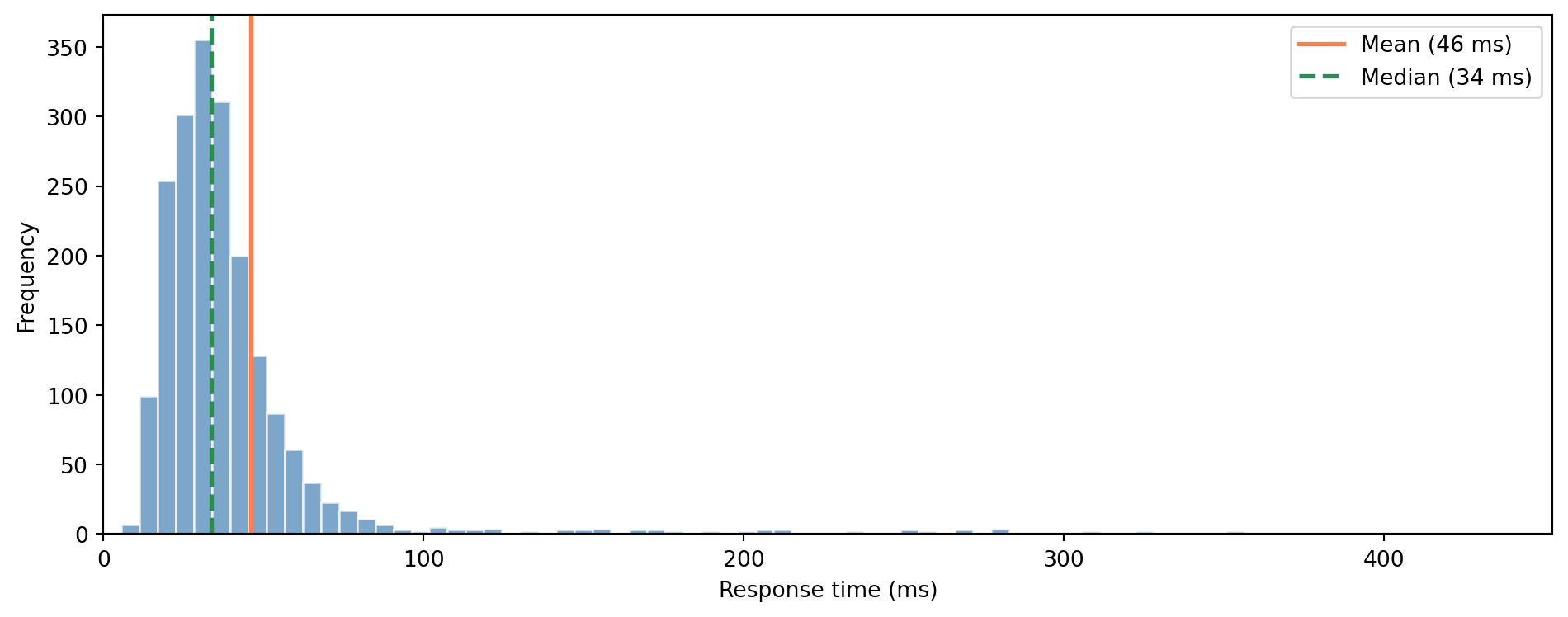
The mean is larger than the median. This is a common indicator of **right skew**, a long tail of slow requests pulling the mean upward, while the median sits where most of the data actually lives. The heuristic works well for distributions like this one, though it's not universally reliable (certain asymmetric distributions can break the pattern). For skewed data, the median is usually the better summary of "typical."
```{python}
#| label: fig-mean-vs-median
#| echo: true
#| fig-cap: "When data is skewed, the mean and median diverge. The mean chases the tail; the median holds the centre."
#| fig-alt: "Histogram of response times showing a right-skewed distribution. A vertical orange line marks the mean, which is pulled rightward by the long tail. A vertical green line marks the median, which sits closer to the bulk of the data. The gap between the two lines illustrates the effect of skewness."
fig, ax = plt.subplots(figsize=(10, 4))
fig.patch.set_alpha(0)
ax.patch.set_alpha(0)

# Clip x-axis to 99.5th percentile so the main distribution shape is visible
x_upper = df['response_time_ms'].quantile(0.995)
ax.hist(df['response_time_ms'], bins=80, edgecolor='white', color='#0072B2',
        alpha=0.7, range=(0, x_upper))
ax.axvline(mean, color='#E69F00', linewidth=2, label=f'Mean ({mean:.0f} ms)')
ax.axvline(median, color='#009E73', linewidth=2, linestyle='--',
           label=f'Median ({median:.0f} ms)')
ax.set_xlabel('Response time (ms)')
ax.set_ylabel('Frequency')
ax.legend()
ax.set_xlim(0, x_upper)
ax.yaxis.grid(True, linestyle=':', alpha=0.4, color='grey')
ax.set_axisbelow(True)
ax.spines['top'].set_visible(False)
ax.spines['right'].set_visible(False)
plt.tight_layout()
plt.show()
```
::: {.callout-note}
## Engineering Bridge
You already know this distinction from latency monitoring. Your p50 latency *is* the median. When your team reports "average response time is 45ms" but users are complaining, it's usually because the *mean* is being pulled up by a tail of slow requests that the median would have filtered out. The SRE (site reliability engineering) rule of thumb — report p50, p95, and p99, not just the average — is descriptive statistics in action. You've been doing this; now you know the formal names.
:::
## Spread: how far from the centre? {#sec-spread}
Knowing the centre isn't enough. Two datasets can have the same mean but completely different character. A service with p50=50ms and p99=55ms is very different from one with p50=50ms and p99=2,000ms, even though their medians match.
The **variance** measures the average squared deviation from the mean:
$$
s^2 = \frac{1}{n-1}\sum_{i=1}^{n} (x_i - \bar{x})^2
$$
The $n-1$ in the denominator (rather than $n$) is called **Bessel's correction**. Think of **degrees of freedom** as the number of independent pieces of information in your data — once you've fixed the mean from $n$ values, only $n-1$ of them can vary freely (the last one is determined by the constraint that they must average to $\bar{x}$). We've "used up" one degree of freedom estimating the mean, so we divide by $n-1$ to avoid systematically underestimating the variance. The more data you have, the less this one-unit adjustment matters relative to $n$.
::: {.callout-tip}
## Author's Note
Why square the deviations instead of just taking the absolute value? It's a natural question, and both approaches are valid: the **mean absolute deviation** exists and is sometimes used. The squared version won out because it's differentiable everywhere (which matters for optimisation), decomposes neatly into additive components (which matters for ANOVA and regression), and connects directly to the normal distribution (which matters for inference). But nothing about the concept of "spread" *requires* squaring. The variance is a convention that became load-bearing. The entire statistical framework we'll build on later assumes it.
:::
Note the convention: $\sigma$ denotes the population standard deviation (a fixed but unknown parameter) while $s$ denotes the sample standard deviation (our estimate of $\sigma$). Likewise $\sigma^2$ vs $s^2$ for the variance.
The **standard deviation** is the square root of the variance: $s = \sqrt{s^2}$. It's in the same units as the original data, which makes it more interpretable: "the standard deviation is 15ms" means more than "the variance is 225ms²."
The **interquartile range** (IQR) is the distance between the 25th and 75th percentiles. It measures the spread of the middle 50% of the data, ignoring the tails entirely. For skewed data or data with outliers, it's often more informative than the standard deviation.
When comparing spread across variables with very different scales, the **coefficient of variation** ($CV = s / \bar{x}$) normalises the standard deviation by the mean. A CV of 0.5 means the standard deviation is half the mean, regardless of units, useful when you're comparing, say, response times for endpoints that operate at 20ms versus 500ms.
```{python}
#| label: spread-measures
#| echo: true
data = df['response_time_ms']

# ddof = "delta degrees of freedom": 1 means divide by (n-1), 0 by n.
# pandas .std() and .var() use ddof=1 (Bessel's correction) by default.
# numpy .std() and .var() use ddof=0 — a common gotcha when switching between them.
print(f"Standard deviation: {data.std():.1f} ms   (ddof=1)")
print(f"Variance:           {data.var():.1f} ms²  (ddof=1)")
print(f"IQR:                {data.quantile(0.75) - data.quantile(0.25):.1f} ms")
print(f"Range:              {data.min():.1f} – {data.max():.1f} ms")
```
## Shape: beyond centre and spread {#sec-shape}
Two numbers, a measure of centre and a measure of spread, go a long way. But they can't tell the whole story. Two datasets can have identical means and standard deviations but look completely different.
**Skewness** measures asymmetry. A skewness of zero means the distribution is symmetric (like a normal). Positive skewness means a right tail (like our response times). Negative skewness means a left tail.
**Kurtosis** measures the heaviness of the tails relative to a normal distribution. High excess kurtosis means extreme values are more probable than under a normal; the metric is dominated by the tails rather than the peak, so it is best read as a measure of tail heaviness, not "peakedness". In practice, this means your p99.9 latency is much further from the median than a normal distribution would predict.
```{python}
#| label: shape-measures
#| echo: true
data = df['response_time_ms']

# bias=True is the default (biased estimator); for n=2,000 the difference
# from the unbiased version is negligible.
print(f"Skewness: {stats.skew(data):.2f}")
print(f"Kurtosis: {stats.kurtosis(data):.2f} (excess, relative to normal)")
```
Positive skewness confirms what we saw in the histogram: a right tail. The positive excess kurtosis tells us the tails are heavier than a normal distribution's. (The `stats.kurtosis()` function returns *excess* kurtosis, the raw kurtosis minus 3, so that a normal distribution gives zero. This is the default convention in most Python libraries.) Both are signs that assuming normality would be a mistake.
But numbers alone only go so far. The most powerful tool in descriptive statistics is simply *looking at the data*.
```{python}
#| label: fig-visual-summary
#| echo: true
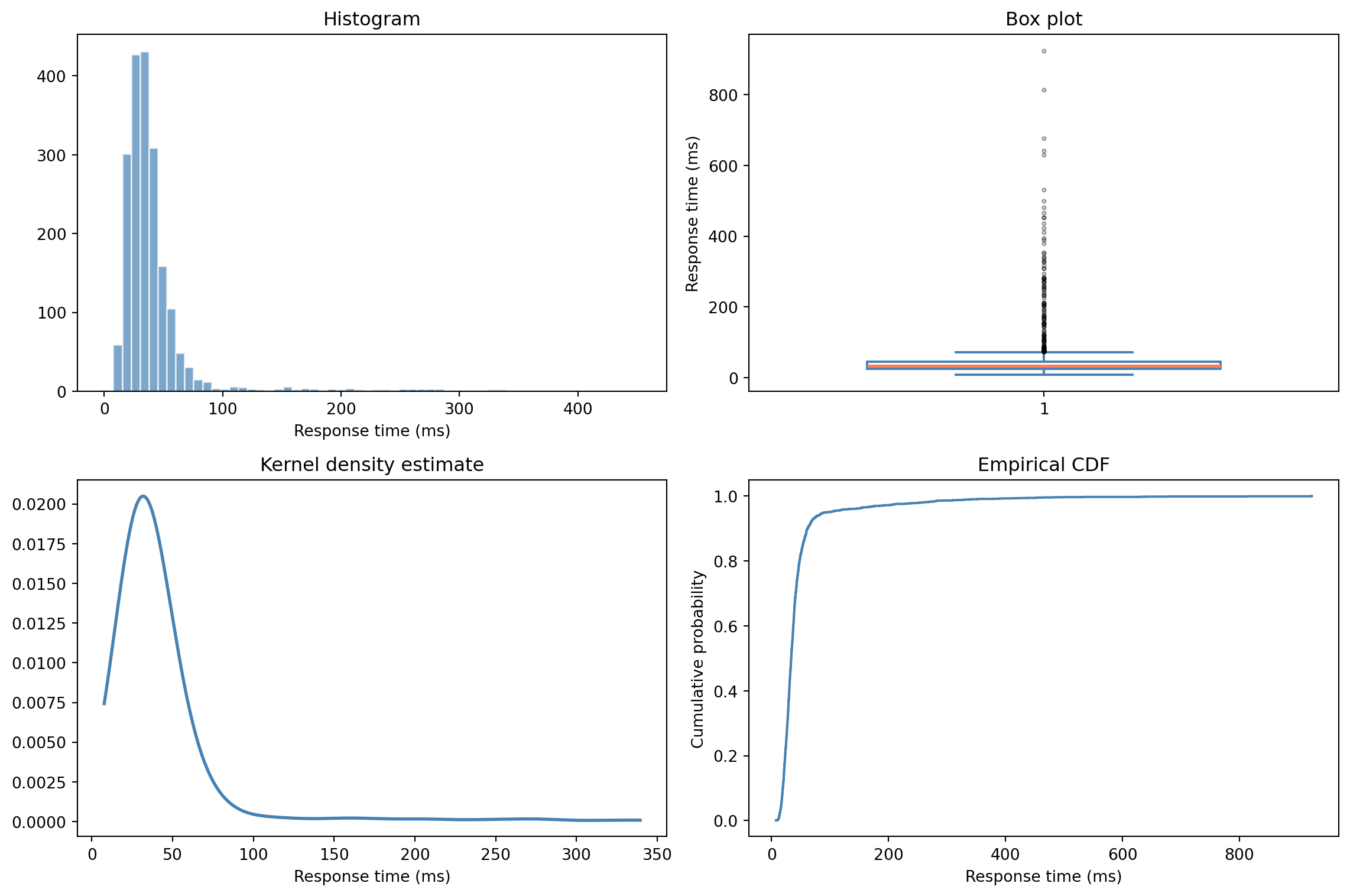
#| fig-cap: "Four views of the same data. The histogram shows shape, the box plot shows quartiles and outliers, the KDE smooths the distribution, and the ECDF (empirical CDF) shows the cumulative picture."
#| fig-alt: "Four-panel figure. Top-left: histogram showing a right-skewed distribution with a main peak and a long tail of slow requests. Top-right: box plot highlighting the median, IQR, and many outlier dots in the right tail. Bottom-left: smooth KDE curve mirroring the histogram shape. Bottom-right: ECDF as a step function rising from 0 to 1, showing percentiles directly on the y-axis."
fig, axes = plt.subplots(2, 2, figsize=(12, 8))
fig.patch.set_alpha(0)
data = df['response_time_ms']

# Histogram — clip range to 99.5th percentile for readability
x_upper = data.quantile(0.995)
axes[0, 0].hist(data, bins=60, edgecolor='white', color='#0072B2', alpha=0.7,
                range=(0, x_upper))
axes[0, 0].set_title('Histogram')
axes[0, 0].set_xlabel('Response time (ms)')

# Box plot — whiskers extend to 1.5×IQR (matplotlib default), not to min/max
axes[0, 1].boxplot(data, widths=0.6,
                   boxprops=dict(color='#0072B2', linewidth=1.5),
                   whiskerprops=dict(color='#0072B2', linewidth=1.5),
                   capprops=dict(color='#0072B2', linewidth=1.5),
                   medianprops=dict(color='#E69F00', linewidth=2),
                   flierprops=dict(marker='.', markersize=4, alpha=0.4))
axes[0, 1].set_title('Box plot')
axes[0, 1].set_ylabel('Response time (ms)')

# KDE (kernel density estimate) — truncated at 99th percentile for readability
x_range = np.linspace(data.min(), data.quantile(0.99), 300)
kde = stats.gaussian_kde(data)
axes[1, 0].plot(x_range, kde(x_range), color='#0072B2', linewidth=2)
axes[1, 0].set_title('Kernel density estimate')
axes[1, 0].set_xlabel('Response time (ms)')

# ECDF (empirical cumulative distribution function)
sorted_data = np.sort(data)
ecdf = np.arange(1, len(sorted_data) + 1) / len(sorted_data)
axes[1, 1].step(sorted_data, ecdf, where='post', color='#0072B2', linewidth=1.5)
axes[1, 1].set_title('Empirical CDF')
axes[1, 1].set_xlabel('Response time (ms)')
axes[1, 1].set_ylabel('Cumulative probability')

for ax in axes.flat:
    ax.patch.set_alpha(0)
    ax.spines['top'].set_visible(False)
    ax.spines['right'].set_visible(False)
    ax.yaxis.grid(True, linestyle=':', alpha=0.4, color='grey')
    ax.set_axisbelow(True)

plt.tight_layout()
plt.show()
```
Each of these plots reveals something different. The **histogram** shows the raw shape — the right skew and the long tail of slow requests are immediately visible. The **box plot** shows the quartiles (Q1, median, Q3), with whiskers extending to $1.5 \times \text{IQR}$ (or the most extreme data point within that range) and values beyond the whiskers flagged as individual outliers. The **KDE** (kernel density estimate) smooths the histogram into a continuous curve, making shape easier to compare across groups. And the **ECDF** (empirical CDF) gives you the cumulative picture: you can read off percentiles directly from the y-axis.
The ECDF deserves special attention because it connects directly to the CDF we met in @sec-pmf-pdf-cdf. The ECDF *is* the CDF estimated from data, a step function that increases by $\frac{1}{n}$ for each observation (or by $\frac{k}{n}$ when $k$ observations share the same value). As $n$ grows, it converges to the true CDF of the underlying distribution.
## The five-number summary {#sec-five-number}
The **five-number summary** — minimum, Q1 (25th percentile), median, Q3 (75th percentile), maximum — is the skeleton of a box plot and a remarkably efficient description of a distribution.
```{python}
#| label: five-number
#| echo: true
data = df['response_time_ms']

summary = {
    'Min': data.min(),
    'Q1 (25th)': data.quantile(0.25),
    'Median (50th)': data.quantile(0.50),
    'Q3 (75th)': data.quantile(0.75),
    'Max': data.max(),
}

for label, value in summary.items():
    print(f"  {label:>15}: {value:>8.1f} ms")

print(f"\n  {'IQR':>15}: {summary['Q3 (75th)'] - summary['Q1 (25th)']:>8.1f} ms")
```
From these five numbers you can read off the centre (median), the spread (IQR), the skewness (compare the distances from Q1 to median vs median to Q3), and the range of the data. The box plot in @fig-visual-summary encodes the quartiles directly; the whiskers mark the range of non-outlier data ($1.5 \times \text{IQR}$ from Q1 and Q3), and points beyond the whiskers appear individually.
This $1.5 \times \text{IQR}$ rule gives you a simple outlier detector: any point beyond $Q_1 - 1.5 \times \text{IQR}$ or $Q_3 + 1.5 \times \text{IQR}$ is flagged. It's not the only approach; you could also use z-scores ($(x - \bar{x}) / s$), which measure how many standard deviations a value lies from the mean. But the IQR method is more robust to the very outliers you're trying to detect, since IQR isn't affected by extreme values the way the standard deviation is. In practice, the hard question is never "how do I detect outliers?" but "is this a genuine extreme value or bad data?" — a question only domain knowledge can answer.
## Relationships between variables {#sec-relationships}
So far we've profiled one variable at a time: location, spread, shape. But real investigations almost always involve asking how two quantities move together. Does response time increase with payload size? Do error rates correlate with deployment frequency? The **correlation coefficient** quantifies linear association between two variables.
The intuition is straightforward. If two variables tend to be above their respective means at the same time (and below them at the same time), they're positively correlated. If one tends to be high when the other is low, they're negatively correlated. We can make this concrete with four made-up pairs of payload size and response time, in (kB, ms): $(1, 100)$, $(3, 140)$, $(5, 180)$, $(7, 220)$. The mean payload is $4$ kB and the mean response is $160$ ms. For each pair, take the deviation of $x$ from its mean and the deviation of $y$ from its mean, and multiply them:
$$
(-3)(-60) = 180, \quad (-1)(-20) = 20, \quad (1)(20) = 20, \quad (3)(60) = 180
$$
Every product is positive because every pair sits above or below both means together — the two variables move in step. Sum the products and you get $400$. If the variables were independent, positive and negative products would cancel out around zero. If they moved inversely (one high when the other low), the sum would be negative. This running total of products-of-deviations carries the raw signal of how $x$ and $y$ co-move; dividing it by $n - 1$ gives the **covariance** (here $400 / 3 \approx 133$).
**Pearson's $r$** is the covariance rescaled to be unitless and bounded between $-1$ and $+1$:
$$
r = \frac{\sum_{i=1}^{n}(x_i - \bar{x})(y_i - \bar{y})}{\sqrt{\sum_{i=1}^{n}(x_i - \bar{x})^2} \cdot \sqrt{\sum_{i=1}^{n}(y_i - \bar{y})^2}}
$$
The numerator is the sum of products of deviations we just computed by hand; the denominator rescales it by the spread of each variable, turning a quantity whose size depends on the units of $x$ and $y$ into one that lives on a fixed scale. The factor of $1/(n-1)$ that turns the numerator into the covariance is matched by the same factor hidden in each standard deviation, so it cancels — equivalently, $r = \text{Cov}(x,y) / (s_x \cdot s_y)$, where $\text{Cov}(x,y) = \frac{1}{n-1}\sum(x_i - \bar{x})(y_i - \bar{y})$ and $s_x$, $s_y$ are the sample standard deviations. In code:
```{python}
#| label: pearson-manual
#| echo: true
# Pearson's r computed manually vs numpy shortcut
# Same four (payload, response) pairs we worked by hand above
x = np.array([1, 3, 5, 7])
y = np.array([100, 140, 180, 220])

r_manual = np.sum((x - x.mean()) * (y - y.mean())) / (
    np.sqrt(np.sum((x - x.mean())**2)) * np.sqrt(np.sum((y - y.mean())**2))
)
r_numpy = np.corrcoef(x, y)[0, 1]

print(f"Manual:  {r_manual:.4f}")
print(f"np.corrcoef: {r_numpy:.4f}")
```
**Spearman's $\rho$** measures *monotonic* (consistently increasing or consistently decreasing) association, regardless of whether the relationship is linear. You compute it by ranking the data and applying Pearson's formula to the ranks. It's more robust to outliers and to monotonic nonlinear relationships, but it still won't detect non-monotonic patterns like the U-shape in the second panel below.
```{python}
#| label: fig-correlation-demo
#| echo: true
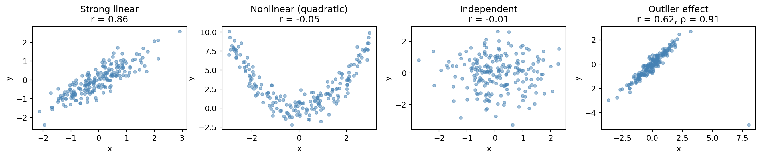
#| fig-cap: "Four datasets with different correlation structures. Pearson's r only captures linear relationships, and a single outlier can drag it down while Spearman's rho, based on ranks, stays robust."
#| fig-alt: "Four scatter plots. First: strong positive linear relationship with r near 0.9. Second: clear quadratic U-shape but near-zero Pearson r, showing r misses nonlinear patterns. Third: random scatter with r near zero. Fourth: strong linear trend disrupted by one extreme outlier, showing Pearson's r drops substantially while Spearman's rho is barely affected."
rng = np.random.default_rng(42)
n = 200

fig, axes = plt.subplots(1, 4, figsize=(14, 3))
fig.patch.set_alpha(0)

# Strong linear
x1 = rng.normal(0, 1, n)
y1 = 0.8 * x1 + rng.normal(0, 0.4, n)
axes[0].scatter(x1, y1, alpha=0.5, s=15, color='#0072B2')
axes[0].set_title(f"Strong linear\nr = {np.corrcoef(x1, y1)[0,1]:.2f}")

# Nonlinear (quadratic)
x2 = rng.uniform(-3, 3, n)
y2 = x2**2 + rng.normal(0, 1, n)
axes[1].scatter(x2, y2, alpha=0.5, s=15, color='#0072B2')
axes[1].set_title(f"Nonlinear (quadratic)\nr = {np.corrcoef(x2, y2)[0,1]:.2f}")

# No relationship — use a fresh seed so the sample correlation is near zero
rng_indep = np.random.default_rng(123)
x3 = rng_indep.normal(0, 1, n)
y3 = rng_indep.normal(0, 1, n)
axes[2].scatter(x3, y3, alpha=0.5, s=15, color='#0072B2')
axes[2].set_title(f"Independent\nr = {np.corrcoef(x3, y3)[0,1]:.2f}")

# Strong but with outlier
x4 = rng.normal(0, 1, n)
y4 = 0.9 * x4 + rng.normal(0, 0.3, n)
x4 = np.append(x4, 8)  # Single extreme outlier
y4 = np.append(y4, -5)
r_pearson = np.corrcoef(x4, y4)[0, 1]
r_spearman = stats.spearmanr(x4, y4).statistic
axes[3].scatter(x4, y4, alpha=0.5, s=15, color='#0072B2')
axes[3].set_title(f"Outlier effect\nr = {r_pearson:.2f}, ρ = {r_spearman:.2f}")

for ax in axes:
    ax.patch.set_alpha(0)
    ax.set_xlabel('x')
    ax.set_ylabel('y')
    ax.spines['top'].set_visible(False)
    ax.spines['right'].set_visible(False)

plt.tight_layout()
plt.show()
```
The second panel is the critical lesson: a clear relationship (quadratic) that Pearson's $r$ completely misses because it's not linear. The fourth panel shows a single outlier dragging Pearson's $r$ down, while Spearman's $\rho$ (based on ranks) is barely affected. Always *plot* the relationship before trusting a correlation number.
One more essential point: **correlation is not causation**. A strong correlation between $x$ and $y$ tells you they move together. It does not tell you that $x$ causes $y$, that $y$ causes $x$, or that some third variable $z$ is driving both. You've seen this in incident investigations — CPU usage correlates with error rate, but a traffic spike causes both. Memory usage and response time both climb during business hours, but request volume is the **confounding variable**. A confounding variable is a hidden third factor that drives both quantities, making them appear related when neither actually causes the other. We'll revisit this properly in *A/B testing: deploying experiments*, where controlled experiments let us establish causation.
## Worked example: profiling a service's performance data {#sec-worked-example-profiling}
Let's put the full toolkit together. Imagine you're investigating performance degradation in a backend service. You have response time data segmented by endpoint.
```{python}
#| label: worked-example-data
#| echo: true
rng = np.random.default_rng(123)  # Fresh RNG for the worked example

n_per_group = 500
endpoints = []
times = []

# /api/users — fast, tight distribution (lognormal for realistic right skew)
endpoints.extend(['/api/users'] * n_per_group)
times.extend(rng.lognormal(mean=3.0, sigma=0.3, size=n_per_group))

# /api/search — slower, more variable
endpoints.extend(['/api/search'] * n_per_group)
times.extend(rng.lognormal(mean=4.0, sigma=0.5, size=n_per_group))

# /api/reports — slow, heavy tail (database-bound)
endpoints.extend(['/api/reports'] * n_per_group)
times.extend(rng.lognormal(mean=5.0, sigma=0.8, size=n_per_group))

perf = pd.DataFrame({
    'endpoint': endpoints,
    'response_time_ms': times
})

# Group-level descriptive stats
perf.groupby('endpoint')['response_time_ms'].describe().round(1)
```
```{python}
#| label: fig-worked-example-comparison
#| echo: true
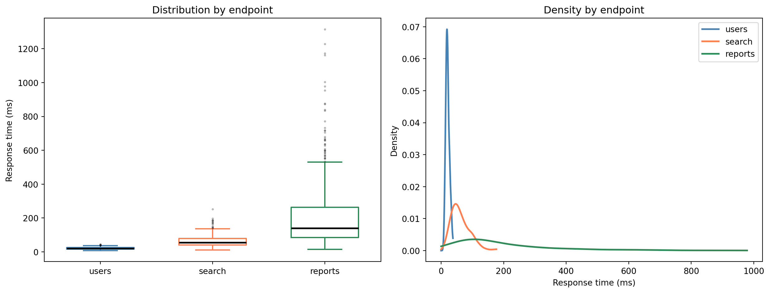
#| fig-cap: "Box plots and KDEs side by side reveal that the three endpoints have fundamentally different performance profiles, not just different averages."
#| fig-alt: "Two-panel figure. The left panel shows three box plots, one per API endpoint. The /api/users endpoint has a tight, low distribution; /api/search is wider and higher; /api/reports has the highest values and the longest tail of outliers. The right panel shows KDE curves for the same three endpoints, drawn with distinct line styles (solid, dashed, dotted), confirming the increasing spread and rightward shift."
fig, (ax1, ax2) = plt.subplots(1, 2, figsize=(13, 5))
fig.patch.set_alpha(0)

# Box plots by endpoint
endpoint_order = ['/api/users', '/api/search', '/api/reports']
colours = {'/api/users': '#0072B2', '/api/search': '#E69F00', '/api/reports': '#009E73'}

for i, ep in enumerate(endpoint_order):
    subset = perf[perf['endpoint'] == ep]['response_time_ms']
    bp = ax1.boxplot(subset, positions=[i], widths=0.6,
                     boxprops=dict(color=colours[ep], linewidth=1.5),
                     whiskerprops=dict(color=colours[ep], linewidth=1.5),
                     capprops=dict(color=colours[ep], linewidth=1.5),
                     medianprops=dict(color='black', linewidth=2),
                     flierprops=dict(marker='.', markersize=3, alpha=0.3))

ax1.set_xticks(range(len(endpoint_order)))
ax1.set_xticklabels([ep.split('/')[-1] for ep in endpoint_order])
ax1.set_ylabel('Response time (ms)')
ax1.set_title('Distribution by endpoint')

# KDEs by endpoint (truncated at 99th percentile for readability).
# Distinct line styles so the curves are distinguishable without colour.
linestyles = {'/api/users': '-', '/api/search': '--', '/api/reports': ':'}
for ep in endpoint_order:
    subset = perf[perf['endpoint'] == ep]['response_time_ms']
    x_range = np.linspace(0, subset.quantile(0.99), 300)
    kde = stats.gaussian_kde(subset)
    ax2.plot(x_range, kde(x_range), linewidth=2, label=ep.split('/')[-1],
             color=colours[ep], linestyle=linestyles[ep])

ax2.set_xlabel('Response time (ms)')
ax2.set_ylabel('Density')
ax2.set_title('Density by endpoint')
ax2.legend()

for ax in (ax1, ax2):
    ax.patch.set_alpha(0)
    ax.spines['top'].set_visible(False)
    ax.spines['right'].set_visible(False)
    ax.yaxis.grid(True, linestyle=':', alpha=0.4, color='grey')
    ax.set_axisbelow(True)

plt.tight_layout()
plt.show()
```
```{python}
#| label: worked-example-quantiles
#| echo: true
# The numbers your SRE team actually cares about
for ep in ['/api/users', '/api/search', '/api/reports']:
    subset = perf[perf['endpoint'] == ep]['response_time_ms']
    print(f"{ep}")
    print(f"  p50: {subset.quantile(0.50):>8.1f} ms")
    print(f"  p95: {subset.quantile(0.95):>8.1f} ms")
    print(f"  p99: {subset.quantile(0.99):>8.1f} ms")
    print(f"  p99/p50 ratio: {subset.quantile(0.99) / subset.quantile(0.50):>5.1f}x")
    print()
```
That p99/p50 ratio is revealing. For `/api/users`, the 99th percentile is roughly 2× the median — a tight, well-behaved distribution. For `/api/reports`, it's far larger — a long tail that means the worst-case experience is dramatically worse than the typical one. The *shape* of the distribution matters as much as its centre. A single "average response time" number would obscure exactly the information you need to prioritise.
Two caveats worth noting. First, descriptive statistics treats your dataset as a bag of unordered values. If your data has a time dimension — and most operational data does — you also need to watch for trends and shifts. A mean computed over a week-long window could mask a gradual degradation that started on Wednesday. Second, aggregating across segments can actively mislead: overall performance might look stable even as one endpoint degrades, because the faster endpoints dominate the aggregate. We'll see this phenomenon formalised as Simpson's paradox in *A/B testing: deploying experiments*.
::: {.callout-note}
## Engineering Bridge
Observability platforms like Grafana, Datadog, and Honeycomb pre-compute percentiles, histograms, and tail latencies for you — but they aggregate over fixed time windows, and you can't average percentiles across windows (the p99 of p99s is *not* the overall p99). When you need to slice data differently — by endpoint, customer segment, or deployment cohort — the tools in this chapter let you compute exactly the summaries you need, from the raw data, rather than relying on what your platform chose to pre-aggregate.
:::
::: {.callout-tip}
## Author's Note
There's a strong temptation to skip straight to modelling. Descriptive statistics feels like "just looking at the data," not real work. But the modelling chapters ahead will make one thing painfully clear: garbage in, garbage out. A histogram that reveals a spike at zero (missing-data sentinels masquerading as measurements) or a scatterplot that exposes a nonlinear relationship saves you from building elaborate models on flawed assumptions. The five minutes you spend profiling a dataset before modelling are the highest-leverage five minutes in the entire workflow.
:::
## Summary {#sec-descriptive-summary}
1. **Descriptive statistics is data profiling** — it's the essential first step before any modelling, answering "what does this data look like?" before you ask "what does it mean?"
2. **Location, spread, and shape tell different stories** — the mean and median tell you where the centre is, the standard deviation and IQR tell you how variable the data is, and skewness and kurtosis tell you about asymmetry and tail behaviour.
3. **Always visualise** — no set of summary statistics can substitute for actually looking at the data. Histograms, box plots, KDEs, and ECDFs each reveal different aspects of the distribution.
4. **Correlation measures linear (or monotonic) association, not causation** — and a single outlier or nonlinear relationship can make Pearson's $r$ misleading. Plot first, compute second.
5. **You already do this** — percentile monitoring and latency dashboards are descriptive statistics. Now you can apply the same toolkit to any dataset, not just the ones your observability platform pre-computes.
## Exercises {#sec-descriptive-exercises}
1. Generate 1,000 samples from a standard normal distribution and compute the mean, median, standard deviation, and IQR. Now add a single outlier at 100. Recompute all four measures. Which ones changed dramatically? What does this tell you about their robustness?
2. Using `rng = np.random.default_rng(42)`, generate two variables: `payload_kb = rng.lognormal(mean=3, sigma=1, size=500)` and `response_ms = 10 + 0.5 * payload_kb + rng.normal(0, 15, size=500)`. Compute both Pearson and Spearman correlations. Now add five outlier points where `payload_kb` is very large but `response_ms` is small (e.g., cached responses for large payloads). How do the two correlation measures react to the outliers? Which would you trust for this data?
3. Load [Anscombe's quartet](https://en.wikipedia.org/wiki/Anscombe%27s_quartet) using `import seaborn as sns; sns.load_dataset('anscombe')`. For each of the four datasets, compute the mean, standard deviation, and Pearson correlation — then plot all four as scatter plots. The summary statistics are nearly identical; the plots are not. What point does this make about the limits of summary statistics?
4. **Conceptual:** This chapter draws a parallel between descriptive statistics and observability tooling (percentile dashboards, latency profiling). Identify two ways in which profiling a *dataset* for modelling differs from profiling a *running service*, and explain why each difference makes the data science version harder.